Rugby World Cup explainer using data

Last week, a stereotypical “French” ceremony opened the 10th Rugby World Cup in Stade de France, in the suburbs of Paris, France. As a small boy growing up in the southern half of France, I developed a strong interest for the sport. Now being an adult living and working in North America, where barely anyone has ever heard the word “Rugby”, I now rarely have anyone else to talk to about Antoine Dupont’s (captain of the French team and best Player in the world in 2021) prowess. Despite being very aware of this reality, I still wasn’t expecting the confused looks on my teammates faces when I casually brought up that I was excited for the World Cup to start during a Friday team meeting. I quickly stopped, before anyone asked more, all too aware that the confusion would only get worse if I had to start saying out loud scores like this 82-8 Ireland blowout or this 32-26 nail-biter involving Wales and Fiji.
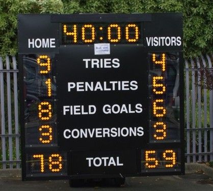
From Rugby Noise. I have to admit that those numbers could look confusing at first

If you squinted at those numbers, keep reading! Sure, those might sound weird at first, but experiencing actions like this score is worth it! In this quick article, I’ll try to give you some explanations and comparisons to other sports grounded in data. Hopefully, in just a few minutes, you’ll be able to join in rugby gossip. And as a bonus, maybe you’ll learn a few things about data analytics in R along the way?
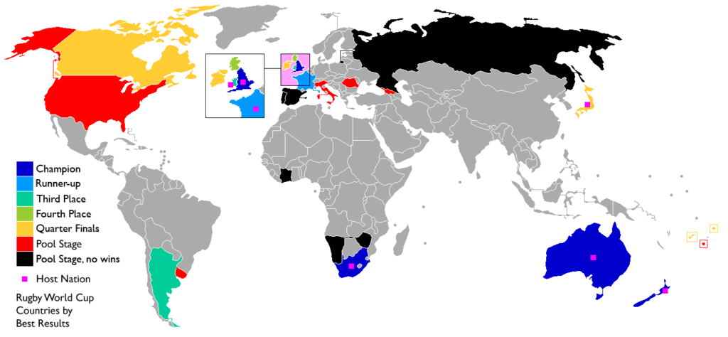
Countries having participated in at least one Rugby World Cup, from Wikipedia

Descriptive data on games scores

First things first, if you don’t know how points are scored in Rugby, I recommend you take a look at this guide. Now, about the data. I have access to a dataset of all International games played between the 19th Century and 2020. Since both how the game is played and how points are scored changed a lot throughout the years, I restricted my dataset to games played since 1995 (close to 1,500 games total). The data and the code are available on GitHub. We can start with some descriptive statistics about scores. Our dataset contains offense, which is the number of points scored by the home team, and diff, the difference with their opponents points (so a negative number means the away team was victorious, and vice versa).

library(tidyverse)
df_sports_with_rugby <- readRDS("df_sports_with_rugby.rds")
desc_stats <- df_sports_with_rugby %>%
  group_by(sport) %>%
  summarize(avg_offense = mean(offense)
        	, med_offense = median(offense)
        	, sd_offense = sd(offense)
        	, avg_diff = mean(diff)
        	, med_diff = median(diff)
        	, sd_diff = sd(diff)
        	) %>%
  arrange(avg_offense %>% desc)
desc_stats
sportavg_offensemed_offensesd_offenseavg_diffmed_diff
basketball102.6510210.982.573.0
rugby33.593016.006.866.0
football27.212708.042.482.5
hockey3.7741.430.271.0
soccer2.0721.330.501.0

As expected, basketball is the sport with the highest average and median winning scores. Rugby and football are fairly close to each other in that regard… which could give the impression that the score will look similar (Spoiler alert: they’re not!). Finally, standard deviations are not necessarily easy to read at first glance, but we immediately spot that despite having an average winner’s points 4 times below basketball’s, it’s standard deviation is higher. And Rugby is also an outlier in score difference. It has actually the highest average, median and standard deviation for diff. So clearly Rugby games are not expected to be close! Highest-level basketball and football on the other hand have an average score difference of just 2.5 points, which is below what you can get in just one action. This hints at very close games with exciting money time… so American! Finally, hockey and soccer have the lowest scores, and their average and median difference is also less than a goal.

One thing that I’d like you to notice is the difference between median and average scores (first two columns of the table above). The two numbers are extremely close for all sports… except Rugby. This suggests that something specific is happening at the tail of the distribution. To get confirmation, we can look at two additional metrics that give us more information about said tail. Skewness, when positive, indicates that accumulation is stronger above the median (below if negative). Kurtosis compares the size of the tail to that of the normal distribution: positive if the tail is larger and negative if lower. A large tail indicates that extreme events (in this case high total points scored) are more likely to happen compared to a variable whose distribution is normal.
In order to compute these two statistics in R, we’ll need the help of another package:

library(e1071)
tail_stats <- df_sports_with_rugby %>%
  group_by(sport) %>%
  summarize( skew_offense = skewness(offense)
        	, kurtosis_offense = kurtosis(offense)
        	, skew_diff = skewness(abs(diff))
        	, kurtosis_diff = kurtosis(abs(diff))
  ) %>%
  arrange(kurtosis_offense)
tail_stats
sportskew_offensekurtosis_offenseskew_diff
football0.14-0.151.26
basketball0.250.361.45
hockey0.460.401.18
soccer0.941.441.24
rugby1.785.502.01

Unsurprisingly, Rugby scores the highest in skewness and kurtosis for total points and point difference. All the other results are very interesting, and a little counter-intuitive. I would not have guessed that soccer would be second to last in that list ordered by tail size, with higher skewness and kurtosis for points and difference than hockey. However, finding football and basketball at the top only confirms the “American” bias towards close games. We can even notice that the Kurtosis of points scored in American football is negative, which makes it a “platykurtic” distribution. In other terms, we’d get a slightly wider total scores table if we simulated football scores from a normal distribution compared to reality. Finally, all the skewnesses of diff are positive. This means a clear accumulation on the positive side of the curve, which is where the home team prevails. In other terms, our 5 sports show signs of home field advantage. Neat.
We can also use ggplot2 to visualize these distributions, for example the home team score (offense):

adjust_offense <- 3 ## Visual factor to adjust smoothness of density
plot_distributions_offense <- ggplot(data=df_sports_with_rugby) +
  geom_density(alpha=0.3, aes(x=offense, fill=sport), adjust=adjust_offense) +
  # scale_x_log10() +
  scale_colour_gradient() +
  labs(x = 'Home team points', y='Density'
   	, title = 'Density plots of home team points') +
  theme_bw() +
  NULL
print(plot_distributions_offense)
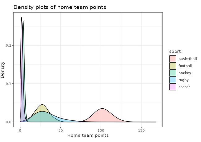
An interesting thing to plot is to focus specifically on football, and compare with a simulated normal distribution, which will show in dashed lines:

football_avg <- desc_stats[desc_stats$sport == 'football',]$avg_offense
football_sd <- desc_stats[desc_stats$sport == 'football',]$sd_offense
adjust_football <- 1.5
plot_distributions_offense_football <- ggplot(data=df_sports_with_rugby %>%
                                   	filter(sport == 'football')) +
  geom_density(alpha=0.3, aes(x=offense, fill=sport), adjust=adjust_football) +
  # scale_x_log10() +
  scale_colour_gradient() +
  labs(x = 'Home team points', y='Density'
   	, title = 'Density plots of home team points') +
  theme_bw() +
  geom_density(data=tibble(t=1:10000, x=rnorm(10000, football_avg, football_sd))
         	,aes(x=x), alpha=0.6, linetype='longdash', adjust=2) +
  NULL
print(plot_distributions_offense_football)
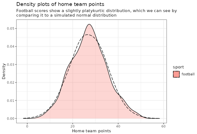
Notice how the distribution peaks higher than normal, and then (at least on the left side), plunges to 0 more quickly than the dashed line? This is negative kurtosis visualized for you. The left and right sides being on different sides of the dashed lines: this one is the positive skewness we noticed a few paragraphs ago.

Converting scores in other sports equivalents

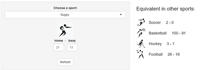
A few years ago, we created a scores converter app, which used comparisons between distributions to propose “equivalent scores” in different sports. Using my new Rugby dataset, all I had to do was add it to the app, and voila… we are now able to play with the app with Rugby and “translate” some of the confusing first round scores I mentioned in my opening paragraph into other sports in which we might be more fluent:
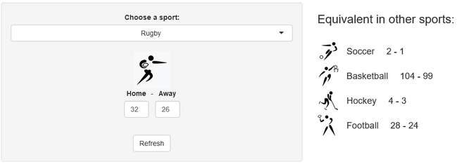
Equivalent scores for Wales-Fiji (32-26)
Equivalent scores for Ireland – Romania (82-8)
Equivalent scores for France – New Zealand (27-13)

I’ll try to keep updating the new scores conversions as the World Cup progresses in our Mastodon and my personal (brand new) Threads. If you have any questions or just want to say hi, feel free to reach out there as well. Happy Rugby World Cup!


Have you checked your features distributions lately?

tl;dr 
Trying to debug a poorly performing machine learning model, I discovered that the distribution of one of the features varied from one date to another. I used a simple and neat affine rescaling. This simple quality improvement brought down the model’s prediction error by a factor 8

Data quality trumps any algorithm

I was recently working on a cool dataset that looked unusually friendly. It was tidy, neat, interesting… the kind of things that you rarely encounter in the wild! My goal was to build a super simple predictor for one of the features. However, I kept getting poor results and at first couldn’t figure out what was happening.

Data sets in tutorials are always cute, data sets in the wild are monstrous
Data sets in tutorials vs data sets in the wild. From Towards AI on Twitter

Here is the dataset I was working with. I tweaked the ids and dates, and muddied the variables a little to make sure I’m not leaking any critical info, but the gist of the problem is absolutely identical to what I was working with (i.e. it’s a real-world datasetTM, not a toy example).

library(tidyverse)
## Load data
data_magictransfo <- readRDS("data/nc233_rescaling_df_04_2021.rds")

This dataset features 211 distinct units and 3 main variables (X1, X2, Y) describing them. We have values for these variables on 7 consecutive dates.

> length(unique(data_magictransfo$unit_id))
[1] 211
> table(data_magictransfo$date_num)

  1   2   3   4   5   6   7 
204 211 211 211 211 211 211

Y is the variable we’re interested in predicting, and we’ll use X1 and X2 as predictors. Since this is basically a problem of machine learning on time series, we’ll use the last date as test set, and train our predictor on the first 6 dates. Usual stuff. To measure the accuracy, we will use the ratio between the square root of the MSE and the mean of the true variable for the 7th date:

df_train <- data_magictransfo %>%  filter(date_num <= 6)
df_test <- data_magictransfo %>%
  filter(date_num > 6)

pred_error_ratio <- function(predict_Y, true_Y) {
 
  mse_rescale <- (predict_Y - true_Y)**2
  mse_rescale <- mean(mse_rescale)
  pred_error_ratio <- sqrt(mse_rescale) / mean(true_Y)
 
  return(pred_error_ratio)
}

The first thing I tried was a super simple linear regression:

simple_model <- lm(Y ~ X1 + X2, data=df_train)
df_test$Y_predict_lm <- predict(simple_model, newdata = df_test)

pred_error_ratio_lm <- pred_error_ratio(df_test$Y_predict_lm, df_test$Y)
> pred_error_ratio_lm
[1] 0.3352261

This extra simple model gives a 33% error rate. Not catastrophic, but not great. Literature on this dataset suggests that 5% should be easily obtained though. Maybe the poor performance comes from the simplicity of the model? Let’s fire up some neural networks and see:

library(nnet)

set.seed(1005192119)
nn <- nnet(Y ~ X1+X2, data=df_train %>% select(Y,X1,X2)
             , size=11, decay=1.0e-5, maxit=5000, linout=T)

df_test$Y_predict_nn <- predict(nn, newdata=df_test %>% select(Y,X1,X2), type="raw")
prediction_error_ratio_nn <- pred_error_ratio(df_test$Y_predict_nn, df_test$Y)
> prediction_error_ratio_nn
[1] 0.1481201

Stop cutting corners and start doing what should always be done first: explore the data

¯\_(ツ)_/¯ Definitely far from what I expected. At this point, I should probably stop cutting corners and start doing what should always be done first: explore the data. After a few summaries, I start suspecting that X1 hides a dirty little secret:

density_plot1 <- ggplot(df_train, aes(x=X1, color=date_num)) +  
  geom_density(fill="lightblue", alpha=0.25) +
  NULL
print(density_plot1)
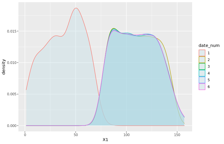
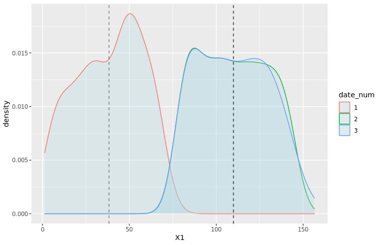
Distribution (density plot) of X1 by date. We see that X1 is clearly sampled from a different distribution for dates 1 and 2
Distribution of X1 by date. X1 is clearly sampled from a different distribution for dates 1 and 2. All dates after 3 show identical distributions

It seems like the distribution of X1 is different between dates 1, 2 and the rest of the dataset! 😱 Let’s zoom in on the first three dates and add vertical dashed lines for the average of X1 by date:

# Add averages to viz
moments_df <- df_train %>%
  filter(date_num <= 3) %>%
  group_by(date_num) %>%
  summarize(mu = mean(X1), sd = sd(X1))
mu_vec <- moments_df$mu

density_plot3 <- ggplot(df_train %>% filter(date_num <= 3), aes(x=X1, color=date_num)) +
  geom_density(fill="lightblue", alpha=0.25) +
  geom_vline(xintercept=mu_vec, linetype="dashed", color="black", alpha=0.5) +
  NULL
print(density_plot3)
Distribution of X1 for dates 1, 2 and 3
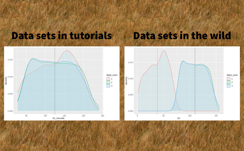
Distribution of X1 for dates 1, 2 and 3. Shapes are different for all three dates but averages for dates 2 and 3 are identical

Clearly, X1 for date 1 is a wildly different thing than other dates. At date 2, the distribution is closer to what it will be in the future: average is very close, but there is still a clear difference in the shape and the width of the tails.

As a data scientist, it’s your job to investigate the data-generating process 🕵️

This problem of features having different distributions by date (or by any other grouping than time, which could very well be possible as well) is common and can arise for multiple reasons. As a data scientist, it’s your job to investigate the data-generating process 🕵️ In this case, X1 comes from a score a certain authority attributes to each unit. A quick investigation revealed that the scoring method used had changed between dates 1 and 2, and then another time between dates 2 and 3. The change only affected the score and not the rank of the units, which means a simple fix should do 🙌

Now that we’ve diagnosed the problem, let’s try and fix it! Let’s open the math toolbox and… No, don’t go away! I promise it will be simple! 😂 The simplest tool in the box will suffice at first. We’ll try a rescaling of the form:

\( Z = a X_1 + b \)


The expected value and variance of this new variable are easy to compute using well-know formulae:

\( E(Z) = a E(X_1) + b \\ Var(Z) = a^2 Var(X_1) \)


We want the rescaled variable Z to have the same average and variance as the distribution from date 3 onwards. Let’s denote them μ and σ2. We thus have:

\( \mu = a \cdot E(X_1) + b \\ \sigma^2 = a^2 \cdot Var(X_1) \)


Since we know E(X1) and Var(X1) from the data, this is actually a very simple linear system with two variables (a and b) and two equations. The unique solution is:

\( a = \frac{\sigma}{Var(X_1)}\\ b = \mu ~ – ~ \frac{\sigma}{Var(X_1)} \cdot E(X_1) \)


which we can now apply on our data:

# Distribution parameters
library(zeallot) # Only used to improve code readability

moments2_df <- df_train %>% 
   mutate(date_select = case_when(
     date_num == "1" ~ "1",
     date_num == "2" ~ "2",
     date_num >= "3" ~ "3+",
     TRUE ~ "NA")
   ) %>% 
   select(date_select, X1) %>% 
   group_by(date_select) %>% 
   summarise(mu=mean(X1), sigma=sd(X1))

c(mu_1, mu_2, mu_Z) %<-% moments2_df$mu
c(sigma_1, sigma_2, sigma_Z) %<-% moments2_df$sigma
 
df_train <- df_train %>%
  mutate(X1_rescale = case_when(
    date_num == 1 ~ a1 * X1 + b1,
    date_num == 2 ~ a2 * X1 + b2,
    TRUE ~ X1
  ))

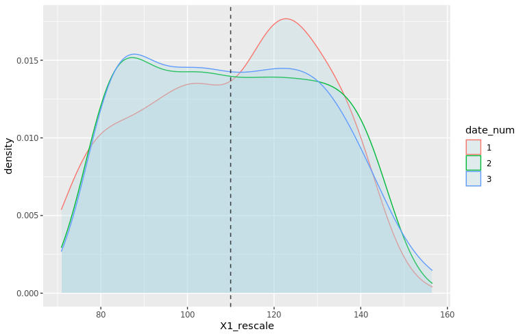
The new density plots look much better!

moments_df_rescale <- df_train %>%  filter(date_num <= 3) %>%
  group_by(date_num) %>%
  summarize(mu = mean(X1_rescale), sd = sd(X1_rescale))
mu_vec_rescale <- moments_df_rescale$mu

density_plot4 <- ggplot(df_train %>% filter(date_num <= 3), aes(x=X1_rescale, color=date_num)) +
  geom_density(fill="lightblue", alpha=0.25) +
  geom_vline(xintercept=mu_vec_rescale, linetype="dashed", color="black", alpha=0.5) +
  NULL
print(density_plot4)
Density plots of rescaled variables
Distribution (density) of rescaled X1 for dates 1, 2 and 3. The distributions are now centered on the same average and have same width

Now we can train our models on the rescaled data:

# New predictions
simple_model_rescale <- lm(Y ~ X1_rescale + X2, data=df_train)

df_test$X1_rescale <- df_test$X1
df_test$Y_predict_rescale <- predict(simple_model_rescale, newdata = df_test)
pred_error_ratio_rescale <- pred_error_ratio(df_test$Y_predict_rescale, df_test$Y)


set.seed(1005192119)
nn_check <- nnet(Y ~ X1_rescale+X2, data=df_train %>% select(Y,X1_rescale,X2)
           , size=13, decay=1.0e-5, maxit=5000, linout=T)

Y_predict_nn_check <- predict(nn_check, newdata=df_test %>% select(Y,X1_rescale,X2), type="raw")
prediction_error_ratio_nn_check <- pred_error_ratio(Y_predict_nn_check, df_test$Y)

The prediction errors go down by a lot! 🎉🎉🎉 8% for the linear model and 2.6% for the neural network:

> pred_error_ratio_rescale
[1] 0.08092733
> prediction_error_ratio_nn_check
[1] 0.02650212

As always, data quality trumps any algorithm, as powerful as it may be!
And lesson learned for me: never trust a cute-looking dataset. Data in the wild is always hard to tame.


To be continued…


Do you like data science and would be interested in building products that help entrepreneurs around the world start and grow their businesses? Shopify is hiring 2021 engineers and data scientists worldwide! Feel free to reach out if you’d like to know more 🙂

Causal Inference cheat sheet for data scientists

Being able to make causal claims is a key business value for any data science team, no matter their size.
Quick analytics (in other words, descriptive statistics) are the bread and butter of any good data analyst working on quick cycles with their product team to understand their users. But sometimes some important questions arise that need more precise answers. Business value sometimes means distinguishing what is true insights from what is incidental noise. Insights that will hold up versus temporary marketing material. In other terms causation.

When answering these questions, absolute rigour is required. Failing to understand key mechanisms could mean missing out on important findings, rolling out the wrong version of a product, and eventually costing your business millions of dollars, or crucial opportunities.
Ron Kohavi, former director of the experimentation team at Microsoft, has a famous example: changing the place where credit card offers were displayed on amazon.com generated millions in revenue for the company.

The tech industry has picked up on this trend in the last 6 years, making Causal Inference a hot topic in data science. Netflix, Microsoft and Google all have entire teams built around some variations of causal methods. Causal analysis is also (finally!) gaining a lot of traction in pure AI fields. Having an idea of what causal inference methods can do for you and for your business is thus becoming more and more important.

The causal inference levels of evidence ladder

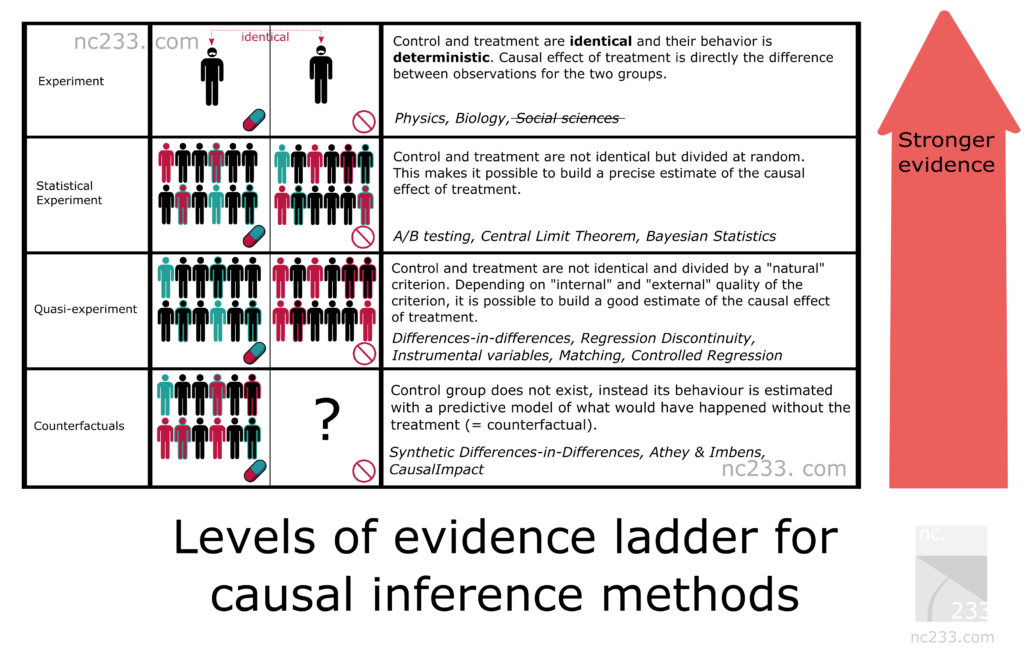
Hence the causal inference ladder cheat sheet! Beyond the value for data scientists themselves, I’ve also had success in the past showing this slide to internal clients to explain how we were processing the data and making conclusions.

The “ladder” classification explains the level of proof each method will give you. The higher, the easier it will be to make sure the results from your methods are true results and reproducible – the downside is that the set-up for the experiment will be more complex. For example, setting up an A/B test typically requires a dedicated framework and engineering resources.
Methods further down the ladder will require less effort on the set-up (think: observational data), but more effort on the rigour of the analysis. Making sure your analysis has true findings and is not just commenting some noise (or worse, is plain wrong) is a process called robustness checks. It’s arguably the most important part of any causal analysis method. The further down on the ladder your method is, the more robustness checks I’ll require if I’m your reviewer 🙂

I also want to stress that methods on lower rungs are not less valuable – it’s almost the contrary! They are brilliant methods that allow use of observational data to make conclusions, and I would not be surprised if people like Susan Athey and Guido Imbens, who have made significant contributions to these methods in the last 10 years, were awarded the Nobel prize one of these days!

causal_cheat_sheet
The causal inference levels of evidence ladder – click on the image to enlarge it

Rung 1 – Scientific experiments

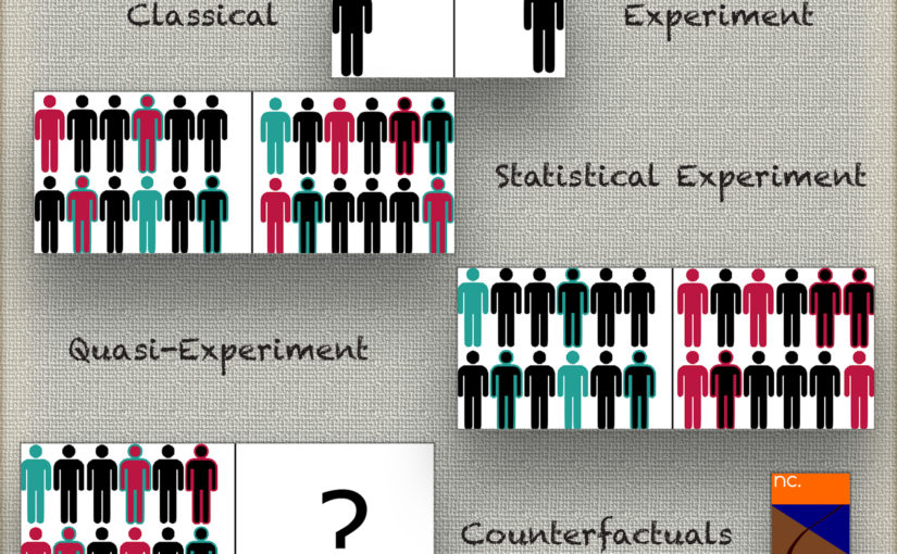
On the first rung of the ladder sit typical scientific experiments. The kind you were probably taught in middle or even elementary school. To explain how a scientific experiment should be conducted, my biology teacher had us take seeds from a box, divide them into two groups and plant them in two jars. The teacher insisted that we made the conditions in the two jars completely identical: same number of seeds, same moistening of the ground, etc.
The goal was to measure the effect of light on plant growth, so we put one of our jars near a window and locked the other one in a closet. Two weeks later, all our jars close to the window had nice little buds, while the ones we left in the closet barely had grown at all.
The exposure to light being the only difference between the two jars, the teacher explained, we were allowed to conclude that light deprivation caused plants to not grow.

Sounds simple enough? Well, this is basically the most rigorous you can be when you want to attribute cause. The bad news is that this methodology only applies when you have a certain level of control on both your treatment group (the one who receives light) and your control group (the one in the cupboard). Enough control at least that all conditions are strictly identical but the one parameter you’re experimenting with (light in this case). Obviously, this doesn’t apply in social sciences nor in data science.

Then why do I include it in this article you might ask? Well, basically because this is the reference method. All causal inference methods are in a way hacks designed to reproduce this simple methodology in conditions where you shouldn’t be able to make conclusions if you followed strictly the rules explained by your middle school teacher.

Rung 2 – Statistical Experiments (aka A/B tests)

Probably the most well-known causal inference method in tech: A/B tests, a.k.a Randomized Controlled Trials for our Biostatistics friends. The idea behind statistical experiments is to rely on randomness and sample size to mitigate the inability to put your treatment and control groups in the exact same conditions. Fundamental statistical theorems like the law of large numbers, the Central Limit theorem or Bayesian inference gives guarantees that this will work and a way to deduce estimates and their precision from the data you collect.

Arguably, an Experiments platform should be one of the first projects any Data Science team should invest in (once all the foundational levels are in place, of course). The impact of setting up an experiments culture in tech companies has been very well documented and has earned companies like Google, Amazon, Microsoft, etc. billions of dollars.

Of course, despite being pretty reliable on paper, A/B tests come with their own sets of caveats. This white paper by Ron Kohavi and other founding members of the Experiments Platform at Microsoft is very useful.

Rung 3 – Quasi-Experiments

As awesome as A/B tests (or RCTs) can be, in some situations they just can’t be performed. This might happen because of lack of tooling (a common case in tech is when a specific framework lacks the proper tools to set up an experiment super quickly and the test becomes counter-productive), ethical concerns, or just simply because you want to study some data ex-post. Fortunately for you if you’re in one of those situations, some methods exist to still be able to get causal estimates of a factor. In rung 3 we talk about the fascinating world of quasi-experiments (also called natural experiments).

A quasi-experiment is the situation when your treatment and control group are divided by a natural process that is not truly random but can be considered close enough to compute estimates. In practice, this means that you will have different methods that will correspond to different assumptions about how “close” you are to the A/B test situation. Among famous examples of natural experiments: using the Vietnam war draft lottery to estimate the impact of being a veteran on your earnings, or the border between New Jersey and Pennsylvania to study the effect of minimum wages on the economy.

Now let me give you a fair warning: when you start looking for quasi-experiments, you can quickly become obsessed by it and start thinking about clever data collection in improbable places… Now you can’t say you haven’t been warned 😜 I have more than a few friends who were lured into attracted by a career in econometrics for the sheer love of natural experiments.

Most popular methods in the world of quasi-experiments are: differences-in-differences (the most common one, according to Scott Cunnigham, author of the Causal Inference Mixtape), Regression Discontinuity Design, Matching, or Instrumental variables (which is an absolutely brilliant construct, but rarely useful in practice). If you’re able to observe (i.e. gather data) on all factors that explain how treatment and control are separated, then a simple linear regression including all factors will give good results.

Rung 4 – The world of counterfactuals

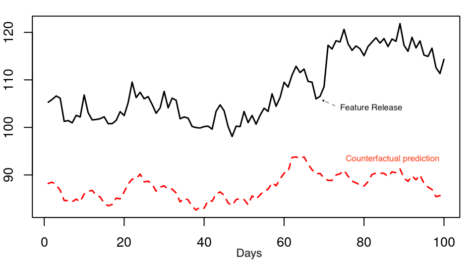
Finally, you will sometimes want to try to detect causal factors from data that is purely observational. A classic example in tech is estimating the effect of a new feature when no A/B test was done and you don’t have any kind of group that isn’t receiving the feature that you could use as a control:

Slightly adapted from CausalImpact‘s documentation

Maybe right new you’re thinking: wait… are you saying we can simply look at the data before and after and be allowed to make conclusions? Well, the trick is that often it isn’t that simple to make a rigorous analysis or even compute an estimate. The idea here is to create a model that will allow to compute a counterfactual control group. Counterfactual means “what would have happened hadn’t this feature existed”. If you have a model of your number of users that you have enough confidence in to make some robust predictions, then you basically have everything

There is a catch though. When using counterfactual methods, the quality of your prediction is key. Without getting too much into the technical details, this means that your model not only has to be accurate enough, but also needs to “understand” what underlying factors are driving what you currently observe. If a confounding factor that is independent from your newest rollout varies (economic climate for example), you do not want to attribute this change to your feature. Your model needs to understand this as well if you want to be able to make causal claims.

This is why robustness checks are so important when using counterfactuals. Some cool Causal Inference libraries like Microsoft’s doWhy do these checks automagically for you 😲 Sensitivity methods like the one implemented in the R package tipr can be also very useful to check some assumptions. Finally, how could I write a full article on causal inference without mentioning DAGs? They are a widely used tool to state your assumptions, especially in the case of rung 4 methods.

(Quick side note: right now with the unprecedented Covid-19 crisis, it’s likely that most prediction models used in various applications are way off. Obviously, those cannot be used for counterfactual causal analysis)

Technically speaking, rung 4 methods look really much like methods from rung 3, with some small tweaks. For example, synthetic diff-in-diff is a combination of diff-in-diff and matching. For time series data, CausalImpact is a very cool and well-known R package. causalTree is another interesting approach worth looking at. More generally, models carefully crafted with domain expertise and rigorously tested are the best tools to do Causal Inference with only counterfactual control groups.

Hope this cheat sheet will help you find the right method for your causal analyses and be impactful for your business! Let us know about your best #causalwins on our Twitter, or in the comments!

[03] La date de Pâques

“Tiens, Pâques est tard l’année prochaine”. Vous avez peut-être aussi déjà entendu cette phrase à propos de Pâques 2017 ? Il est vrai que l’année prochaine, le dimanche pascal aura lieu le 16 avril, soit 20 jours plus tard qu’en 2016 (27 mars). Je me suis demandé quelle était la distribution des dates de Pâques, et quand on pouvait considérer que “Pâques tombe tôt/tard cette année”

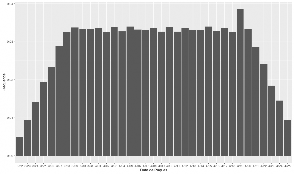
Wikipedia nous informe que “Pâques est le dimanche qui suit le 14e jour de la Lune qui atteint cet âge le 21 mars ou immédiatement après” … ce qui ne nous avance pas beaucoup ! Heureusement, le fameux mathématicien Gauss a établi un algorithme permettant de calculer cette fameuse date avec une suite d’opérations plutôt simples. On obtient alors la fréquence de chaque date, résumée dans ce petit graphe:

Fréquence des dates de Pâques de l'année 1600 à l'année 100000
Fréquence des dates de Pâques de l’année 1600 à l’année 100000

Les résultats, en vrac :

  • Pâques ne peut avoir lieu qu’entre le 22 mars et le 25 avril
  • La date “moyenne” de Pâques est le 8 avril
  • 10% des dimanches de Pâques ont lieu avant le 27 mars (donc on pouvait bien dire qu’en 2016, Pâques tombait tôt !) et 10% après le 20 avril (la prochaine fois, ce sera en 2019, le 21 avril)
  • La date du 19 avril est légèrement plus fréquente que les autres (prochain Pâques à cette date en 2071)
  • Pâques a légèrement plus de chances de tomber un jour impair qu’un jour pair (52% contre 48%)

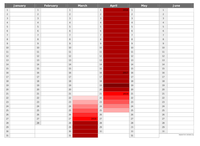
La distribution est résumée de façon plus imagée dans ce petit calendrier :

Distribution de la date de Pâques dans le calendrier. Plus la teinte est rouge, plus la date est fréquente

A demain pour un autre petit article du calendrier de l’avent !