Data analysis of the French football league players with R and FactoMineR

This year we’ve had a great summer for sporting events! Now autumn is back, and with it the Ligue 1 championship. Last year, we created this data analysis tutorial using R and the excellent package FactoMineR for a course at ENSAE (in French). The dataset contains the physical and technical abilities of French Ligue 1 and Ligue 2 players. The goal of the tutorial is to determine with our data analysis which position is best for Mathieu Valbuena 🙂

The dataset

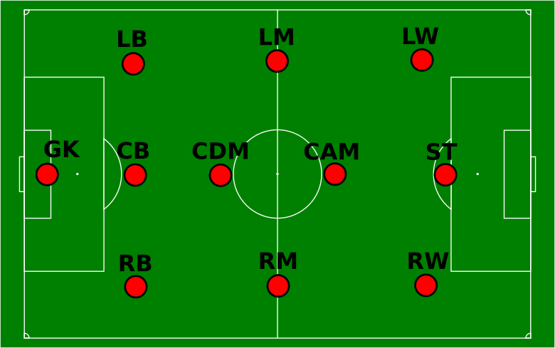
A small precision that could prove useful: it is not required to have any advanced knowledge of football to understand this tutorial. Only a few notions about the positions of the players on the field are needed, and they are summed up in the following diagram:

The data come from the video game Fifa 15 (which is already 2 years old, so there may be some differences with the current Ligue 1 and Ligue 2 players!). The game features rates each players’ abilities in various aspects of the game. Originally, the grade are quantitative variables (between 0 and 100) but we transformed them into categorical variables (we will discuss why we chose to do so later on). All abilities are thus coded on 4 positions : 1. Low / 2. Average / 3. High / 4. Very High.

Loading and prepping the data

Let’s start by loading the dataset into a data.frame. The important thing to note is that FactoMineR requires factors. So for once, we’re going to let the (in)famous stringsAsFactors parameter be TRUE!

> frenchLeague <- read.csv2("french_league_2015.csv", stringsAsFactors=TRUE)
> frenchLeague <- as.data.frame(apply(frenchLeague, 2, factor))

The second line transforms the integer columns into factors also. FactoMineR uses the row.names of the dataframes on the graphs, so we’re going to set the players names as row names:

row.names(frenchLeague) <- frenchLeague$name
frenchLeague$name <- NULL

Here’s what our object looks like (we only display the first few lines here):

> head(frenchLeague)
                     foot position league age height overall
Florian Thauvin      left       RM Ligue1   1      3       4
Layvin Kurzawa       left       LB Ligue1   1      3       4
Anthony Martial     right       ST Ligue1   1      3       4
Clinton N'Jie       right       ST Ligue1   1      2       3
Marco Verratti      right       MC Ligue1   1      1       4
Alexandre Lacazette right       ST Ligue1   2      2       4

Data analysis

Our dataset contains categorical variables. The appropriate data analysis method is the Multiple Correspondance Analysis. This method is implemented in FactoMineR in the method MCA. We choose to treat the variables “position”, “league” and “age” as supplementary:

> library(FactoMineR)
> mca <- MCA(frenchLeague, quali.sup=c(2,3,4))

This produces three graphs: the projection on the factorial axes of categories and players, and the graph of the variables. Let’s just have a look at the second one of these graphs:

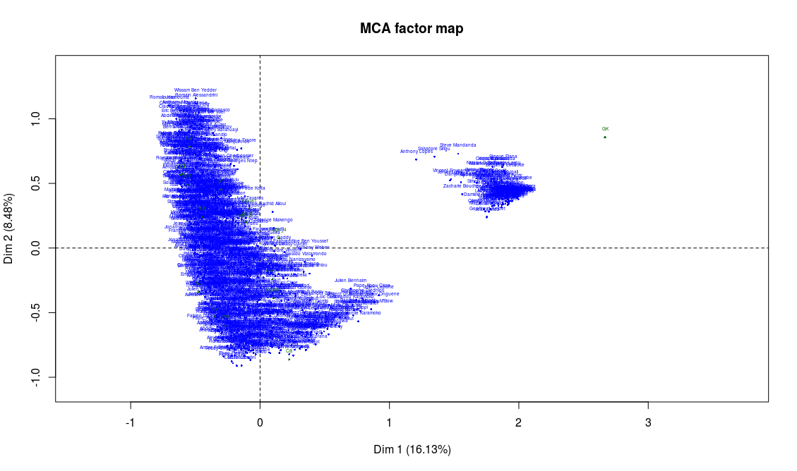
Before trying to go any further into the analysis, something should alert us. There clearly are two clusters of players here! Yet the data analysis techniques like MCA suppose that the scatter plot is homogeneous. We’ll have to restrict the analysis to one of the two clusters in order to continue.

On the previous graph, supplementary variables are shown in green. The only supplementary variable that appears to correspond to the cluster on the right is the goalkeeper position (“GK”). If we take a closer look to the players on this second cluster, we can easily confirm that they’re actually all goalkeeper. This absolutely makes a lot of sense: in football, the goalkeeper is a very different position, and we should expect these players to be really different from the others. From now on, we will only focus on the positions other than goalkeepers. We also remove from the analysis the abilities that are specific to goalkeepers, which are not important for other players and can only add noise to our analysis:

> frenchLeague_no_gk <- frenchLeague[frenchLeague$position!="GK",-c(31:35)]
> mca_no_gk <- MCA(frenchLeague_no_gk, quali.sup=c(2,3,4))

And now our graph features only one cluster.

Interpretation

Obviously, we have to start by reducing the analysis to a certain number of factorial axes. My favorite method to chose the number of axes is the elbow method. We plot the graph of the eigenvalues:

> barplot(mca_no_gk$eig$eigenvalue)

 

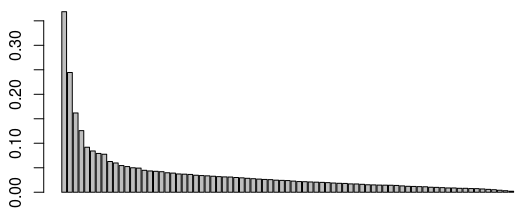
Around the third or fourth eigenvalue, we observe a drop of the values (which is the percentage of the variance explained par the MCA). This means that the marginal gain of retaining one more axis for our analysis is lower after the 3rd or 4th first ones. We thus choose to reduce our analysis to the first three factorial axes (we could also justify chosing 4 axes). Now let’s move on to the interpretation, starting with the first two axes:

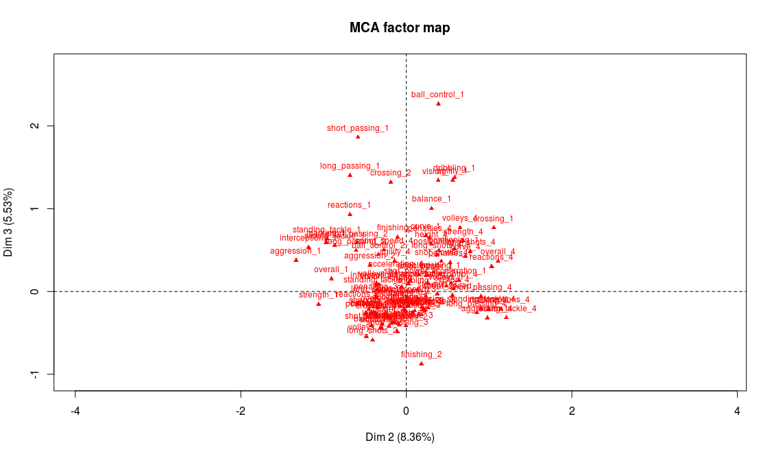
> plot.MCA(mca_no_gk, invisible = c("ind","quali.sup"))

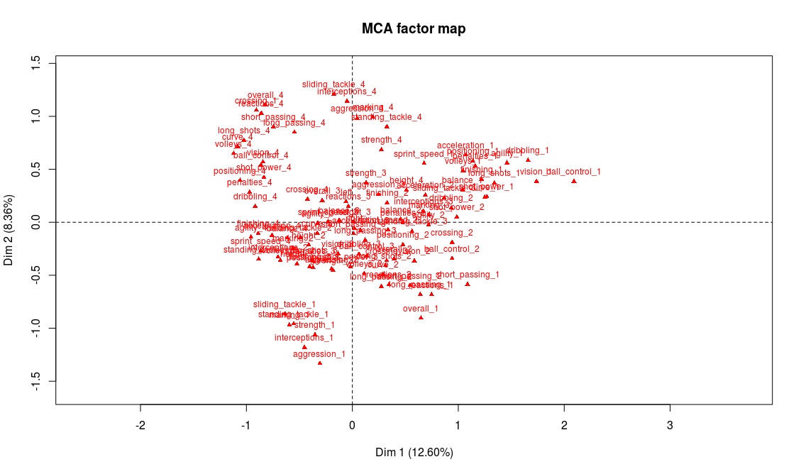
We could start the analysis by reading on the graph the name of the variables and modalities that seem most representative of the first two axes. But first we have to keep in mind that there may be some of the modalities whose coordinates are high that have a low contribution, making them less relevant for the interpretation. And second, there are a lot of variables on this graph, and reading directly from it is not that easy. For these reasons, we chose to use one of FactoMineR’s specific functions, dimdesc (we only show part of the output here):

> dimdesc(mca_no_gk)

$`Dim 1`$category
                      Estimate       p.value
finishing_1        0.700971584 1.479410e-130
volleys_1          0.732349045 8.416993e-125
long_shots_1       0.776647500 4.137268e-111
sliding_tackle_3   0.591937236 1.575750e-106
curve_1            0.740271243  1.731238e-87
[...]
finishing_4       -0.578170467  7.661923e-82
shot_power_4      -0.719591411  2.936483e-86
ball_control_4    -0.874377431 5.088935e-104
dribbling_4       -0.820552850 1.795628e-117

The most representative abilities of the first axis are, on the right side of the axis, a weak level in attacking abilities (finishing, volleys, long shots, etc.) and on the left side a very strong level in those abilities. Our interpretation is thus that axis 1 separates players according to their offensive abilities (better attacking abilities on the left side, weaker on the right side). We procede with the same analysis for axis 2 and conclude that it discriminates players according to their defensive abilities: better defenders will be found on top of the graph whereas weak defenders will be found on the bottom part of the graph.

Supplementary variables can also help confirm our interpretation, particularly the position variable:

> plot.MCA(mca_no_gk, invisible = c("ind","var"))

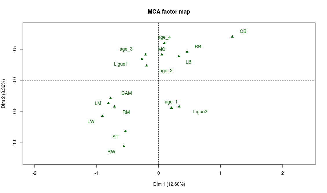
And indeed we find on the left part of the graph the attacking positions (LW, ST, RW) and on the top part of the graph the defensive positions (CB, LB, RB).

If our interpretation is correct, the projection on the second bissector of the graph will be a good proxy for the overall level of the player. The best players will be found on the top left area while the weaker ones will be found on the bottom right of the graph. There are many ways to check this, for example looking at the projection of the modalities of the variable “overall”. As expected, “overall_4” is found on the top-left corner and “overall_1” on the bottom-right corner. Also, on the graph of the supplementary variables, we observe that “Ligue 1” (first division of the french league) is on the top-left area while “Ligue 2” (second division) lies on the bottom-right area.

With only these two axes interpreted there are plenty of fun things to note:

• Left wingers seem to have a better overall level than right wingers (if someone has an explanation for this I’d be glad to hear it!)
• Age is irrelevant to explain the level of a player, except for the younger ones who are in general weaker.
• Older players tend to have more defensive roles

Let’s not forget to deal with axis 3:

> plot.MCA(mca_no_gk, invisible = c("ind","var"), axes=c(2,3))

Modalities that are most representative of the third axis are technical weaknesses: the players with the lower technical abilities (dribbling, ball control, etc.) are on the end of the axis while the players with the highest grades in these abilities tend to be found at the center of the axis:

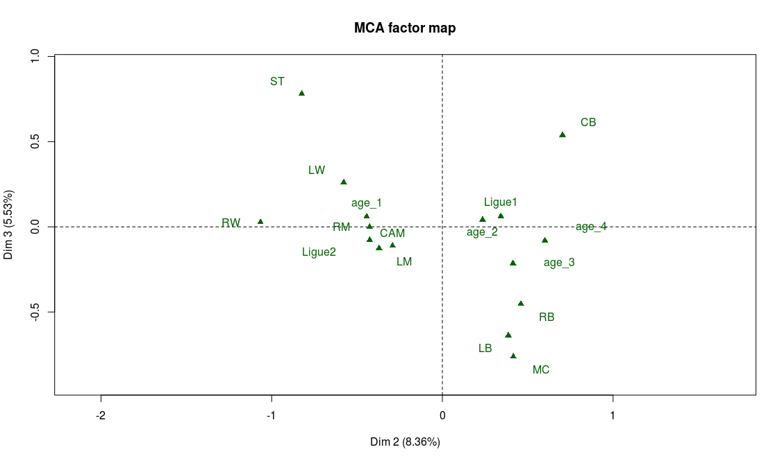
We note with the help of the supplementary variables, that midfielders have the highest technical abilities on average, while strikers (ST) and defenders (CB, LB, RB) seem in general not to be known for their ball control skills.

Now we see why we chose to make the variables categorical instead of quantitative. If we had kept the orginal variables (quantitative) and performed a PCA on the data, the projections would have kept the orders for each variable, unlike what happens here for axis 3. And after all, isn’t it better like this? Ordering players according to their technical skills isn’t necessarily what you look for when analyzing the profiles of the players. Football is a very rich sport, and some positions don’t require Messi’s dribbling skills to be an amazing player!

Mathieu Valbuena

Now we add the data for a new comer in the French League, Mathieu Valbuena (actually Mathieu Valbuena arrived in the French League in August of 2015, but I warned you that the data was a bit old ;)). We’re going to compare Mathieu’s profile (as a supplementary individual) to the other players, using our data analysis.

> columns_valbuena <- c("right","RW","Ligue1",3,1
 ,4,4,3,4,3,4,4,4,4,4,3,4,4,3,3,1,3,2,1,3,4,3,1,1,1)
> frenchLeague_no_gk["Mathieu Valbuena",] <- columns_valbuena

> mca_valbuena <- MCA(frenchLeague_no_gk, quali.sup=c(2,3,4), ind.sup=912)
> plot.MCA(mca_valbuena, invisible = c("var","ind"), col.quali.sup = "red", col.ind.sup="darkblue")
> plot.MCA(mca_valbuena, invisible = c("var","ind"), col.quali.sup = "red", col.ind.sup="darkblue", axes=c(2,3))

Last two lines produce the graphs with Mathieu Valbuena on axes 1 and 2, then 2 and 3:

So, Mathieu Valbuena seems to have good offensive skills (left part of the graph), but he also has a good overall level (his projection on the second bissector is rather high). He also lies at the center of axis 3, which indicates he has good technical skills. We should thus not be surprised to see that the positions that suit him most (statistically speaking of course!) are midfield positions (CAM, LM, RM). With a few more lines of code, we can also find the French league players that have the most similar profiles:

> mca_valbuena_distance <- MCA(frenchLeague_no_gk[,-c(3,4)], quali.sup=c(2), ind.sup=912, ncp = 79)
> distancesValbuena <- as.data.frame(mca_valbuena_distance$ind$coord)
> distancesValbuena[912, ] <- mca_valbuena_distance$ind.sup$coord

> euclidianDistance <- function(x,y) {
 
 return( dist(rbind(x, y)) )
 
}

> distancesValbuena$distance_valbuena <- apply(distancesValbuena, 1, euclidianDistance, y=mca_valbuena_distance$ind.sup$coord)
> distancesValbuena <- distancesValbuena[order(distancesValbuena$distance_valbuena),]

> names_close_valbuena <- c("Mathieu Valbuena", row.names(distancesValbuena[2:6,]))

And we get: Ladislas Douniama, Frédéric Sammaritano, Florian Thauvin, N’Golo Kanté and Wissam Ben Yedder.

There would be so many other things to say about this data set but I think it’s time to wrap this (already very long) article up 😉 Keep in mind that this analysis should not be taken too seriously! It just aimed at giving a fun tutorial for students to discover R, FactoMineR and data analysis.