analytics – NC233

Rugby World Cup explainer using data

Last week, a stereotypical “French” ceremony opened the 10th Rugby World Cup in Stade de France, in the suburbs of Paris, France. As a small boy growing up in the southern half of France, I developed a strong interest for the sport. Now being an adult living and working in North America, where barely anyone has ever heard the word “Rugby”, I now rarely have anyone else to talk to about Antoine Dupont’s (captain of the French team and best Player in the world in 2021) prowess. Despite being very aware of this reality, I still wasn’t expecting the confused looks on my teammates faces when I casually brought up that I was excited for the World Cup to start during a Friday team meeting. I quickly stopped, before anyone asked more, all too aware that the confusion would only get worse if I had to start saying out loud scores like this 82-8 Ireland blowout or this 32-26 nail-biter involving Wales and Fiji.

*From* *Rugby Noise. I have to admit that those numbers could look confusing at first*

If you squinted at those numbers, keep reading! Sure, those might sound weird at first, but experiencing actions like this score is worth it! In this quick article, I’ll try to give you some explanations and comparisons to other sports grounded in data. Hopefully, in just a few minutes, you’ll be able to join in rugby gossip. And as a bonus, maybe you’ll learn a few things about data analytics in R along the way?

Countries having participated in at least one Rugby World Cup, from Wikipedia

Descriptive data on games scores

First things first, if you don’t know how points are scored in Rugby, I recommend you take a look at this guide. Now, about the data. I have access to a dataset of all International games played between the 19th Century and 2020. Since both how the game is played and how points are scored changed a lot throughout the years, I restricted my dataset to games played since 1995 (close to 1,500 games total). The data and the code are available on GitHub. We can start with some descriptive statistics about scores. Our dataset contains offense, which is the number of points scored by the home team, and diff, the difference with their opponents points (so a negative number means the away team was victorious, and vice versa).

library(tidyverse)
df_sports_with_rugby <- readRDS("df_sports_with_rugby.rds")
desc_stats <- df_sports_with_rugby %>%
  group_by(sport) %>%
  summarize(avg_offense = mean(offense)
        	, med_offense = median(offense)
        	, sd_offense = sd(offense)
        	, avg_diff = mean(diff)
        	, med_diff = median(diff)
        	, sd_diff = sd(diff)
        	) %>%
  arrange(avg_offense %>% desc)
desc_stats

sport	avg_offense	med_offense	sd_offense	avg_diff	med_diff
basketball	102.65	102	10.98	2.57	3.0
rugby	33.59	30	16.00	6.86	6.0
football	27.21	27	08.04	2.48	2.5
hockey	3.77	4	1.43	0.27	1.0
soccer	2.07	2	1.33	0.50	1.0

As expected, basketball is the sport with the highest average and median winning scores. Rugby and football are fairly close to each other in that regard… which could give the impression that the score will look similar (Spoiler alert: they’re not!). Finally, standard deviations are not necessarily easy to read at first glance, but we immediately spot that despite having an average winner’s points 4 times below basketball’s, it’s standard deviation is higher. And Rugby is also an outlier in score difference. It has actually the highest average, median and standard deviation for diff. So clearly Rugby games are not expected to be close! Highest-level basketball and football on the other hand have an average score difference of just 2.5 points, which is below what you can get in just one action. This hints at very close games with exciting money time… so American! Finally, hockey and soccer have the lowest scores, and their average and median difference is also less than a goal.

One thing that I’d like you to notice is the difference between median and average scores (first two columns of the table above). The two numbers are extremely close for all sports… except Rugby. This suggests that something specific is happening at the tail of the distribution. To get confirmation, we can look at two additional metrics that give us more information about said tail. Skewness, when positive, indicates that accumulation is stronger above the median (below if negative). Kurtosis compares the size of the tail to that of the normal distribution: positive if the tail is larger and negative if lower. A large tail indicates that extreme events (in this case high total points scored) are more likely to happen compared to a variable whose distribution is normal.
In order to compute these two statistics in R, we’ll need the help of another package:

library(e1071)
tail_stats <- df_sports_with_rugby %>%
  group_by(sport) %>%
  summarize( skew_offense = skewness(offense)
        	, kurtosis_offense = kurtosis(offense)
        	, skew_diff = skewness(abs(diff))
        	, kurtosis_diff = kurtosis(abs(diff))
  ) %>%
  arrange(kurtosis_offense)
tail_stats

sport	skew_offense	kurtosis_offense	skew_diff
football	0.14	-0.15	1.26
basketball	0.25	0.36	1.45
hockey	0.46	0.40	1.18
soccer	0.94	1.44	1.24
rugby	1.78	5.50	2.01

Unsurprisingly, Rugby scores the highest in skewness and kurtosis for total points and point difference. All the other results are very interesting, and a little counter-intuitive. I would not have guessed that soccer would be second to last in that list ordered by tail size, with higher skewness and kurtosis for points and difference than hockey. However, finding football and basketball at the top only confirms the “American” bias towards close games. We can even notice that the Kurtosis of points scored in American football is negative, which makes it a “platykurtic” distribution. In other terms, we’d get a slightly wider total scores table if we simulated football scores from a normal distribution compared to reality. Finally, all the skewnesses of diff are positive. This means a clear accumulation on the positive side of the curve, which is where the home team prevails. In other terms, our 5 sports show signs of home field advantage. Neat.
We can also use ggplot2 to visualize these distributions, for example the home team score (offense):

adjust_offense <- 3 ## Visual factor to adjust smoothness of density
plot_distributions_offense <- ggplot(data=df_sports_with_rugby) +
  geom_density(alpha=0.3, aes(x=offense, fill=sport), adjust=adjust_offense) +
  # scale_x_log10() +
  scale_colour_gradient() +
  labs(x = 'Home team points', y='Density'
   	, title = 'Density plots of home team points') +
  theme_bw() +
  NULL
print(plot_distributions_offense)

An interesting thing to plot is to focus specifically on football, and compare with a simulated normal distribution, which will show in dashed lines:

football_avg <- desc_stats[desc_stats$sport == 'football',]$avg_offense
football_sd <- desc_stats[desc_stats$sport == 'football',]$sd_offense
adjust_football <- 1.5
plot_distributions_offense_football <- ggplot(data=df_sports_with_rugby %>%
                                   	filter(sport == 'football')) +
  geom_density(alpha=0.3, aes(x=offense, fill=sport), adjust=adjust_football) +
  # scale_x_log10() +
  scale_colour_gradient() +
  labs(x = 'Home team points', y='Density'
   	, title = 'Density plots of home team points') +
  theme_bw() +
  geom_density(data=tibble(t=1:10000, x=rnorm(10000, football_avg, football_sd))
         	,aes(x=x), alpha=0.6, linetype='longdash', adjust=2) +
  NULL
print(plot_distributions_offense_football)

Notice how the distribution peaks higher than normal, and then (at least on the left side), plunges to 0 more quickly than the dashed line? This is negative kurtosis visualized for you. The left and right sides being on different sides of the dashed lines: this one is the positive skewness we noticed a few paragraphs ago.

Converting scores in other sports equivalents

A few years ago, we created a scores converter app, which used comparisons between distributions to propose “equivalent scores” in different sports. Using my new Rugby dataset, all I had to do was add it to the app, and voila… we are now able to play with the app with Rugby and “translate” some of the confusing first round scores I mentioned in my opening paragraph into other sports in which we might be more fluent:

*Equivalent scores for Wales-Fiji (32-26)*

*Equivalent scores for Ireland – Romania (82-8)*

*Equivalent scores for France – New Zealand (27-13)*

I’ll try to keep updating the new scores conversions as the World Cup progresses in our Mastodon and my personal (brand new) Threads. If you have any questions or just want to say hi, feel free to reach out there as well. Happy Rugby World Cup!

Causal Inference cheat sheet for data scientists

Being able to make causal claims is a key business value for any data science team, no matter their size.
Quick analytics (in other words, descriptive statistics) are the bread and butter of any good data analyst working on quick cycles with their product team to understand their users. But sometimes some important questions arise that need more precise answers. Business value sometimes means distinguishing what is true insights from what is incidental noise. Insights that will hold up versus temporary marketing material. In other terms causation.

When answering these questions, absolute rigour is required. Failing to understand key mechanisms could mean missing out on important findings, rolling out the wrong version of a product, and eventually costing your business millions of dollars, or crucial opportunities.
Ron Kohavi, former director of the experimentation team at Microsoft, has a famous example: changing the place where credit card offers were displayed on amazon.com generated millions in revenue for the company.

The tech industry has picked up on this trend in the last 6 years, making Causal Inference a hot topic in data science. Netflix, Microsoft and Google all have entire teams built around some variations of causal methods. Causal analysis is also (finally!) gaining a lot of traction in pure AI fields. Having an idea of what causal inference methods can do for you and for your business is thus becoming more and more important.

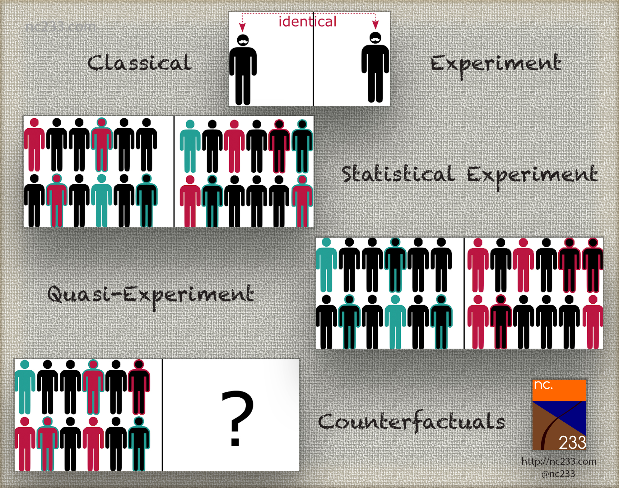
The causal inference levels of evidence ladder

Hence the causal inference ladder cheat sheet! Beyond the value for data scientists themselves, I’ve also had success in the past showing this slide to internal clients to explain how we were processing the data and making conclusions.

The “ladder” classification explains the level of proof each method will give you. The higher, the easier it will be to make sure the results from your methods are true results and reproducible – the downside is that the set-up for the experiment will be more complex. For example, setting up an A/B test typically requires a dedicated framework and engineering resources.
Methods further down the ladder will require less effort on the set-up (think: observational data), but more effort on the rigour of the analysis. Making sure your analysis has true findings and is not just commenting some noise (or worse, is plain wrong) is a process called robustness checks. It’s arguably the most important part of any causal analysis method. The further down on the ladder your method is, the more robustness checks I’ll require if I’m your reviewer 🙂

I also want to stress that methods on lower rungs are not less valuable – it’s almost the contrary! They are brilliant methods that allow use of observational data to make conclusions, and I would not be surprised if people like Susan Athey and Guido Imbens, who have made significant contributions to these methods in the last 10 years, were awarded the Nobel prize one of these days!

causal_cheat_sheet — The causal inference levels of evidence ladder – click on the image to enlarge it

Rung 1 – Scientific experiments

On the first rung of the ladder sit typical scientific experiments. The kind you were probably taught in middle or even elementary school. To explain how a scientific experiment should be conducted, my biology teacher had us take seeds from a box, divide them into two groups and plant them in two jars. The teacher insisted that we made the conditions in the two jars completely identical: same number of seeds, same moistening of the ground, etc.
The goal was to measure the effect of light on plant growth, so we put one of our jars near a window and locked the other one in a closet. Two weeks later, all our jars close to the window had nice little buds, while the ones we left in the closet barely had grown at all.
The exposure to light being the only difference between the two jars, the teacher explained, we were allowed to conclude that light deprivation caused plants to not grow.

Sounds simple enough? Well, this is basically the most rigorous you can be when you want to attribute cause. The bad news is that this methodology only applies when you have a certain level of control on both your treatment group (the one who receives light) and your control group (the one in the cupboard). Enough control at least that all conditions are strictly identical but the one parameter you’re experimenting with (light in this case). Obviously, this doesn’t apply in social sciences nor in data science.

Then why do I include it in this article you might ask? Well, basically because this is the reference method. All causal inference methods are in a way hacks designed to reproduce this simple methodology in conditions where you shouldn’t be able to make conclusions if you followed strictly the rules explained by your middle school teacher.

Rung 2 – Statistical Experiments (aka A/B tests)

Probably the most well-known causal inference method in tech: A/B tests, a.k.a Randomized Controlled Trials for our Biostatistics friends. The idea behind statistical experiments is to rely on randomness and sample size to mitigate the inability to put your treatment and control groups in the exact same conditions. Fundamental statistical theorems like the law of large numbers, the Central Limit theorem or Bayesian inference gives guarantees that this will work and a way to deduce estimates and their precision from the data you collect.

Arguably, an Experiments platform should be one of the first projects any Data Science team should invest in (once all the foundational levels are in place, of course). The impact of setting up an experiments culture in tech companies has been very well documented and has earned companies like Google, Amazon, Microsoft, etc. billions of dollars.

Of course, despite being pretty reliable on paper, A/B tests come with their own sets of caveats. This white paper by Ron Kohavi and other founding members of the Experiments Platform at Microsoft is very useful.

Rung 3 – Quasi-Experiments

As awesome as A/B tests (or RCTs) can be, in some situations they just can’t be performed. This might happen because of lack of tooling (a common case in tech is when a specific framework lacks the proper tools to set up an experiment super quickly and the test becomes counter-productive), ethical concerns, or just simply because you want to study some data ex-post. Fortunately for you if you’re in one of those situations, some methods exist to still be able to get causal estimates of a factor. In rung 3 we talk about the fascinating world of quasi-experiments (also called natural experiments).

A quasi-experiment is the situation when your treatment and control group are divided by a natural process that is not truly random but can be considered close enough to compute estimates. In practice, this means that you will have different methods that will correspond to different assumptions about how “close” you are to the A/B test situation. Among famous examples of natural experiments: using the Vietnam war draft lottery to estimate the impact of being a veteran on your earnings, or the border between New Jersey and Pennsylvania to study the effect of minimum wages on the economy.

Now let me give you a fair warning: when you start looking for quasi-experiments, you can quickly become obsessed by it and start thinking about clever data collection in improbable places… Now you can’t say you haven’t been warned 😜 I have more than a few friends who were ~~lured into~~ attracted by a career in econometrics for the sheer love of natural experiments.

Most popular methods in the world of quasi-experiments are: differences-in-differences (the most common one, according to Scott Cunnigham, author of the Causal Inference Mixtape), Regression Discontinuity Design, Matching, or Instrumental variables (which is an absolutely brilliant construct, but rarely useful in practice). If you’re able to observe (i.e. gather data) on all factors that explain how treatment and control are separated, then a simple linear regression including all factors will give good results.

Rung 4 – The world of counterfactuals

Finally, you will sometimes want to try to detect causal factors from data that is purely observational. A classic example in tech is estimating the effect of a new feature when no A/B test was done and you don’t have any kind of group that isn’t receiving the feature that you could use as a control:

Slightly adapted from CausalImpact‘s documentation

Maybe right new you’re thinking: wait… are you saying we can simply look at the data before and after and be allowed to make conclusions? Well, the trick is that often it isn’t that simple to make a rigorous analysis or even compute an estimate. The idea here is to create a model that will allow to compute a counterfactual control group. Counterfactual means “what would have happened hadn’t this feature existed”. If you have a model of your number of users that you have enough confidence in to make some robust predictions, then you basically have everything

There is a catch though. When using counterfactual methods, the quality of your prediction is key. Without getting too much into the technical details, this means that your model not only has to be accurate enough, but also needs to “understand” what underlying factors are driving what you currently observe. If a confounding factor that is independent from your newest rollout varies (economic climate for example), you do not want to attribute this change to your feature. Your model needs to understand this as well if you want to be able to make causal claims.

This is why robustness checks are so important when using counterfactuals. Some cool Causal Inference libraries like Microsoft’s doWhy do these checks automagically for you 😲 Sensitivity methods like the one implemented in the R package tipr can be also very useful to check some assumptions. Finally, how could I write a full article on causal inference without mentioning DAGs? They are a widely used tool to state your assumptions, especially in the case of rung 4 methods.

(Quick side note: right now with the unprecedented Covid-19 crisis, it’s likely that most prediction models used in various applications are way off. Obviously, those cannot be used for counterfactual causal analysis)

Technically speaking, rung 4 methods look really much like methods from rung 3, with some small tweaks. For example, synthetic diff-in-diff is a combination of diff-in-diff and matching. For time series data, CausalImpact is a very cool and well-known R package. causalTree is another interesting approach worth looking at. More generally, models carefully crafted with domain expertise and rigorously tested are the best tools to do Causal Inference with only counterfactual control groups.

Hope this cheat sheet will help you find the right method for your causal analyses and be impactful for your business! Let us know about your best #causalwins on our Twitter, or in the comments!

Est-ce que cette piscine est bien notée ?

J’ai pris la (mauvaise ?) habitude d’utiliser Google Maps et son système de notation (chaque utilisateur peut accorder une note de une à cinq étoiles) pour décider d’où je me rend : restaurants, lieux touristiques, etc. Récemment, j’ai déménagé et je me suis intéressé aux piscines environnantes, pour me rendre compte que leur note tournait autour de 3 étoiles. Je me suis alors fait la réflexion que je ne savais pas, si, pour une piscine, il s’agissait d’une bonne ou d’une mauvaise note ! Pour les restaurants et bars, il existe des filtres permettant de se limiter dans sa recherche aux établissements ayant au moins 4 étoiles ; est-ce que cela veut dire que cette piscine est très loin d’être un lieu de qualité ? Pourtant, dès lors qu’on s’intéresse à d’autres types de services comme les services publics, ou les hôpitaux, on se rend compte qu’il peut y avoir de nombreux avis négatifs, et des notes très basses, par exemple :

Pour répondre à cette question, il faudrait connaître les notes qu’ont les autres piscines pour savoir si 3 étoiles est un bon score ou non. Il serait possible de le faire manuellement, mais ce serait laborieux ! Pour éviter cela, nous allons utiliser l’API de GoogleMaps (Places, vu qu’on va s’intéresser à des lieux et non des trajets ou des cartes personnalisées).

API, késako? Une API est un système intégré à un site web permettant d’y accéder avec des requêtes spécifiques. J’avais déjà utilisé une telle API pour accéder aux données sur le nombre de vues, de like, etc. sur Youtube ; il existe aussi des API pour Twitter, pour Wikipedia…

Pour utiliser une telle API, il faut souvent s’identifier ; ici, il faut disposer d’une clef API spécifique pour Google Maps qu’on peut demander ici. On peut ensuite utiliser l’API de plusieurs façons : par exemple, faire une recherche de lieux avec une chaîne de caractères, comme ici “Piscine in Paris, France” (avec cette fonction) ; ensuite, une fois que l’on dispose de l’identifiant du lieu, on peut chercher plus de détails, comme sa note, avec cette fonction. De façon pratique, j’ai utilisé le package googleway qui possède deux fonctions qui font ce que je décris juste avant : google_place et google_place_details.

En utilisant ces fonctions, j’ai réussi à récupérer de l’information sur une soixantaine de piscines à Paris et ses environs très proches (je ne sais pas s’il s’agit d’une limite de l’API, mais le nombre ne semblait pas aberrant !). J’ai récupéré les notes et je constate ainsi que la note moyenne est autour de 3.5, ce qui laisse à penser que les piscines à proximité de mon nouvel appartement ne sont pas vraiment les meilleures… De façon plus visuelle, je peux ensuite représenter leur note moyenne (en rouge quand on est en dessous de 2, en vert de plus en plus foncé au fur et à mesure qu’on se rapproche de 5) sur la carte suivante (faite avec Leaflet, en utilisant le très bon package leaflet)

Comparaison avec d’autres lieux

En explorant Google Maps aux alentours, je me suis rendu compte que les agences bancaires du quartier étaient particulièrement mal notées, en particulier pour une banque spécifique (dont je ne citerai pas le nom – mais dont le logo est un petit animal roux). Je peux utiliser la même méthode pour récupérer par l’API des informations sur ces agences (et je constate qu’effectivement, la moyenne des notes est de 2 étoiles), puis les rajouter sur la même carte (les piscines correspondent toujours aux petits cercles ; les agences bancaires sont représentées par des cercles plus grands), en utilisant le même jeu de couleurs que précédemment :

La carte est difficile à lire : on remarque surtout que les petits cercles (les piscines) sont verts et que les grands (les agences bancaires) sont rouges. Or, il pourrait être intéressant de pouvoir comparer entre eux les lieux de même type. Pour cela, nous allons séparer au sein des piscines les 20% les moins bien notées, puis les 20% d’après, etc., et faire de même avec les agences bancaires. On applique ensuite un schéma de couleur qui associe du rouge aux 40% des lieux les pires – relativement (40% des piscines et 40% des agences bancaires), et du vert pour les autres. La carte obtenue est la suivante : elle permet de repérer les endroits de Paris où se trouvent, relativement, les meilleurs piscines et les meilleures agences bancaires en un seul coup d’œil !

Google introduit des modifications aux notes (en particulier quand il y a peu de notes, voir ici (en), mais pas seulement (en)) ; il pourrait être intéressant d’ajouter une fonctionnalité permettant de comparer les notes des différents lieux relativement aux autres de même catégorie !

[Sports] Fifa et analyse de données

Après un été chargé en sports, l’automne et la Ligue 1 reprennent peu à peu leurs droits. C’est l’occasion de détailler un sujet d’analyse de données élaboré pour un cours à l’ENSAE. Il s’agit d’analyser des données qualitatives (caractéristiques physiques, tactiques et aptitudes relatives à certains aspects techniques du jeu) décrivant les joueurs du championnat de France de football. Le but final est de déterminer “statistiquement” à quel poste faire jouer Mathieu Valbuena 🙂 On utilise le langage R et l’excellent package d’analyse de données FactoMineR.

Les données

Comme indiqué dans l’énoncé du TD, il n’est pas nécessaire de bien connaître le football pour pouvoir suivre cet article. Seule une notion de l’emplacement des joueurs sur le terrain en fonction de leur poste (correspondant à la colonne “position” du dataset) est souhaitable. Voici un petit schéma pour aider les moins avertis :

Les données sont issues du jeu vidéo Fifa 15 (les connaisseurs auront remarqué que les données datent donc d’il y a déjà deux saisons, il peut donc y avoir quelques différences avec les effectifs actuels !), qui donne de nombreuses statistiques pour chaque joueur, incluant une évaluation de leurs capacités. Les données de Fifa sont quantitatives (par exemple chaque capacité est notée sur 100) mais pour cet article on les a rendues catégorielles sur 4 positions : 1. Faible / 2. Moyen / 3. Fort / 4. Très fort. On verra l’intérêt d’avoir procédé ainsi un peu plus loin !

Préparation des données

Commençons par charger les données. Notez l’utilisation de l’option stringsAsFactors=TRUE (plus d’explications sur ce fameux paramètre stringsAsFactors ici). Eh oui, une fois n’est pas coutume, FactoMineR utilise des facteurs pour effectuer l’analyse de données !

> champFrance <- read.csv2("td3_donnees.csv", stringsAsFactors=TRUE)
> champFrance <- as.data.frame(apply(champFrance, 2, factor))

La deuxième ligne sert à transformer les colonnes de type int créés par read.csv2 en factors.

FactoMineR utilise le paramètre “row.names” des data.frame de R pour l’affichage sur les graphes. On va donc indiquer qu’il faut utiliser la colonne “nom” en tant que row.names pour faciliter la lecture :

> row.names(champFrance) <- champFrance$nom
> champFrance$nom <- NULL

Voilà à quoi ressemble désormais notre data.frame (seules les premières lignes sont affichées) :

> head(champFrance)
                      pied position championnat age taille general
Florian Thauvin     Gauche      MDR      Ligue1   1      3       4
Layvin Kurzawa      Gauche       AG      Ligue1   1      3       4
Anthony Martial      Droit       BU      Ligue1   1      3       4
Clinton N'Jie        Droit       BU      Ligue1   1      2       3
Marco Verratti       Droit       MC      Ligue1   1      1       4
Alexandre Lacazette  Droit       BU      Ligue1   2      2       4

Analyse des données

Nous avons affaire à un tableau de variables catégorielles : la méthode adaptée est l’Analyse des Correspondances Multiples, qui est implémentée dans FactoMineR par la méthode MCA. Pour le moment on exclut de l’analyse les variables “position”, “championnat” et “âge” (que l’on traite comme variables supplémentaires) :

> library(FactoMineR)
> acm <- MCA(champFrance, quali.sup=c(2,3,4))

Trois graphes apparaissent dans la sortie : la projection sur les deux premiers axes factoriels des catégories et des individus, ainsi que le graphe des variables. A ce stade, seul le second nous intéresse :

2_nuages_points_2 — Projection des individus sur les deux premiers axes factoriels

Avant même d’essayer d’aller plus loin dans l’analyse, quelque chose doit nous sauter aux yeux : il y a clairement deux nuages de points ! Or nos méthodes d’analyse de données supposent que le nuage qu’on analyse est homogène. Il va donc falloir se restreindre à l’analyse de l’un des deux nuages que l’on observe sur ce graphe.

Pour identifier à quels individus le nuage de droite correspond, on peut utiliser les variables supplémentaires (points verts). On observe que la projection de la position goal (“G”) correspond bien au nuage. En regardant de plus près les noms des individus concernés, on confirme que ce sont tous des gardiens de but.

On va se concentrer pour le reste de l’article sur les joueurs de champ. On en profite également pour retirer les colonnes ne concernant que les capacités de gardien, qui ne sont pas importantes pour les joueurs de champ et ne peuvent que bruiter notre analyse :

> champFrance_nogoals <- champFrance[champFrance$position!="G",-c(31:35)]
> acm_nogoals <- MCA(champFrance_nogoals, quali.sup=c(2,3,4))

Et l’on vérifie bien dans la sortie graphique que l’on a un nuage de points homogène.

Interprétation

On commence par réduire notre analyse à un certain nombre d’axes factoriels. Ma méthode favorite est la “règle du coude” : sur le graphe des valeurs propres, on va observer un décrochement (le “coude”) suivi d’une décroissance régulière. On sélectionnera ensuite un nombre d’axes correspondant au nombre de valeurs propres précédant le décrochement :

> barplot(acm_nogoals$eig$eigenvalue)

Ici, on peut choisir par exemple 3 axes (mais on pourrait justifier aussi de retenir 4 axes). Passons maintenant à l’interprétation, en commençant par les graphes des projections sur les deux premiers axes retenus pour l’étude.

> plot.MCA(acm_nogoals, invisible = c("ind","quali.sup"))

axes_1_2_modalites — Projection des modalités sur les axes factoriels 1 et 2 (cliquer pour agrandir)

On peut par exemple lire sur ce graphe le nom des modalités possédant les plus fortes coordonnées sur les axes 1 et 2 et commencer ainsi l’interprétation. Mais avec un tel de nombre de modalités, la lecture directe sur le graphe n’est pas si aisée. On peut également obtenir un résultat dans la sortie texte spécifique de FactoMineR, dimdesc (seule une partie de la sortie est donnée ici) :

> dimdesc(acm_nogoals)

$`Dim 1`$category
                         Estimate       p.value
finition_1            0.700971584 1.479410e-130
volees_1              0.732349045 8.416993e-125
tirs_lointains_1      0.776647500 4.137268e-111
tacle_glisse_3        0.591937236 1.575750e-106
effets_1              0.740271243  1.731238e-87
[...]
finition_4           -0.578170467  7.661923e-82
puissance_tir_4      -0.719591411  2.936483e-86
controle_balle_4     -0.874377431 5.088935e-104
dribbles_4           -0.820552850 1.795628e-117

Les modalités les plus caractéristiques de l’axe 1 sont, à droite, un niveau faible dans les capacités offensives (finition, volées, tirs lointains), et de l’autre un niveau très fort dans ces même capacités. L’interprétation naturelle est donc que l’axe 1 discrimine selon les capacités offensives (les meilleurs attaquants à gauche, les moins bons à droite). On procède de même pour l’axe 2, et on observe le même phénomène, mais avec les capacités défensives : en haut on trouvera les meilleurs défenseurs, et en bas les moins bons défenseurs.

Les variables supplémentaires peuvent aussi aider à l’interprétation, et vont confirmer notre interprétation, notamment la variable de position :

> plot.MCA(acm_nogoals, invisible = c("ind","var"))

var_sup_axes_1_2 — Projection des variables supplémentaires sur les axes factoriels 1 et 2 (cliquer pour agrandir)

On trouve bien à gauche du graphe les les postes offensifs (BU, AIG, AID) et en haut les postes défensifs (DC, AD, AG).

Une conséquence de cette interprétation est que l’on risque de trouver les joueurs de meilleur niveau organisés le long de la seconde bissectrice, avec les meilleurs joueurs dans le quadrant en haut à gauche, et les plus faibles dans le quadrant en bas à droite. Il y a beaucoup de moyens de le vérifier, mais on va se contenter de regarder dans le graphe des modalités l’emplacement des observations de la variable “général”, qui résume le niveau d’un joueur. Comme on s’y attend, on trouve “général_4” dans en haut à gauche et “général_1” dans le quadrant en bas à droite. On peut observer aussi le placement des variables supplémentaires “Ligue 1” et “Ligue 2” pour s’en convaincre 🙂

A ce stade, il y a déjà plein de choses intéressantes à relever ! Parmi celles qui m’amusent le plus :

Les ailiers gauches semblent avoir un meilleur niveau que les ailiers droits (si un spécialiste du foot voulait bien m’en expliquer la raison ce serait top !)
L’âge n’est pas explicatif du niveau du joueur, sauf pour les plus jeunes qui ont un niveau plus faible
Les joueurs les plus âgés ont des rôles plus défensifs.

N’oublions pas de nous occuper de l’axe 3 :

> plot.MCA(acm_nogoals, invisible = c("ind","var"), axes=c(2,3))

axes_2_3 — Modalités projetées sur les axes 2 et 3

Les modalités les plus caractéristiques de ce troisième axe sont les faiblesses techniques : les joueurs les moins techniques sont sur les extrémités de l’axe, et les joueurs les plus techniques au centre. On le confirme sur le graphe des variables supplémentaires : les buteurs et défenseurs centraux sont en effet moins réputés pour leurs capacités techniques, tandis que tous les postes de milieux se retrouvent au centre de l’axe :

sup_axes_2_3 — Variables supplémentaires sur les axes 2 et 3 (cliquer pour agrandir)

C’est l’intérêt d’avoir rendu ces variables catégorielles. Si l’on avait conservé le caractère quantitatif des données originelles de Fifa et effectué une ACP, les projections de chaque caractéristique sur chaque axe auraient été ordonnées par niveau, contrairement à ce qui se passe sur l’axe 3. Et après tout, discriminer les joueurs suivant leur niveau technique ne reflète pas forcément toute la richesse du football : à certains postes, on a besoin de techniciens, mais à d’autres, on préférera des qualités physiques !

Mathieu Valbuena

On va maintenant ajouter les données d’un nouvel entrant dans le championnat de France : Mathieu Valbuna (oui je vous avais prévenu, les données commencent à dater un peu :p) et le comparer aux autres joueurs en utilisant notre analyse.

> columns_valbuena <- c("Droit","AID","Ligue1",3,1
 ,4,4,3,4,3,4,4,4,4,4,3,4,4,3,3,1,3,2,1,3,4,3,1,1,1)
> champFrance_nogoals["Mathieu Valbuena",] <- columns_valbuena

> acm_valbuena <- MCA(champFrance_nogoals, quali.sup=c(2,3,4), ind.sup=912)
> plot.MCA(acm_valbuena, invisible = c("var","ind"), col.quali.sup = "red", col.ind.sup="darkblue")
> plot.MCA(acm_valbuena, invisible = c("var","ind"), col.quali.sup = "red", col.ind.sup="darkblue", axes=c(2,3))

Les deux dernières lignes permettent de représenter Mathieu Valbuena sur les axes 1 et 2, puis 2 et 3 :

Axes factoriels 1 et 2 avec Mathieu Valbuena en point supplémentaire (cliquer pour agrandir)

Axes factoriels 2 et 3 avec Mathieu Valbuena en point supplémentaire (cliquer pour agrandir)

Résultat de notre analyse : Mathieu Valbuena a plutôt un profil offensif (gauche de l’axe 1), mais possède un bon niveau général (sa projection sur la deuxième bissectrice est assez élevée). Il possède également de bonnes aptitudes techniques (centre de l’axe 3). Enfin, ses qualités semblent plutôt bien convenir aux postes de milieu offensif (MOC) ou milieu gauche (MG). Avec quelques lignes de code, on peut trouver les joueurs du championnat dont le profil est le plus proche de celui de Valbuena :

> acm_valbuena_distance <- MCA(champFrance_nogoals[,-c(3,4)], quali.sup=c(2), ind.sup=912, ncp = 79)
> distancesValbuena <- as.data.frame(acm_valbuena_distance$ind$coord)
> distancesValbuena[912, ] <- acm_valbuena_distance$ind.sup$coord

> euclidianDistance <- function(x,y) {
 
 return( dist(rbind(x, y)) )
 
}

> distancesValbuena$distance_valbuena <- apply(distancesValbuena, 1, euclidianDistance, y=acm_valbuena_distance$ind.sup$coord)
> distancesValbuena <- distancesValbuena[order(distancesValbuena$distance_valbuena),]

# On regarde les profils des 5 individus les plus proches
> nomsProchesValbuena <- c("Mathieu Valbuena", row.names(distancesValbuena[2:6,]))

Et l’on obtient : Ladislas Douniama, Frédéric Sammaritano, Florian Thauvin, N’Golo Kanté et Wissam Ben Yedder.

Il y aurait plein d’autres choses à dire sur ce jeu de données mais je préfère arrêter là cet article déjà bien long 😉 Pour finir, gardez à l’esprit que cette analyse n’est pas vraiment sérieuse et sert surtout à présenter un exemple sympathique pour la découverte de FactoMineR et de l’ADD.

[Sports] Best/Worst NBA matchups ever

Earlier this month, the Philadelphia 76ers grabbed their first (and for now, only) win of the season by beating the Lakers. That night, checking for the menu on the NBA League Pass, I quickly elected not to watch this pretty unappealing matchup. Though I couldn’t help thinking that it is a shame for franchises that have both won NBA titles and see legends of the game wear their jerseys. During many seasons, a Lakers-Sixers game meant fun, excitement and most important of all excellent basketball. And I started wondering what were the best and worst matchups throughout NBA history.

Data and model

My criterion to evaluate these matchups will be the mean level of the two teams during each season. In fact, by “good” matchup I mean a game that feature two excellent ball clubs, making it an evening every NBA fan awaits impatiently as soon as the season calendar is made available. On the contrary, a “bad” matchup is a game whose only stake will be to determine draft pick orders. My criterion does not predict the actual interest of watching these games: a confrontation between two top teams might very well be pretty boring if the star players are having a bad night (or if the coach decides to bench them). Also, a contest between two mediocre teams might very well finally be a three-OT thriller with players showing excellent basketball skills. In fact, my criterion only holds from an historical perspective (or in the very unlikely case that you have to choose between the replay of several games without knowing when these games were played 🙂 ).

The level of each team is estimated using the excellent FiveThirtyEight NBA Elo rankings. Then, to rank the 435 possible matchups between the 30 NBA franchises, I will average the mean level of every two teams for all years between 1977 and 2015 (I chose to limit the analysis to after the NBA-ABA merger of 1976 so as to avoid dealing with defunct franchises). You can found the R codes I used on my GitHub page.

The best matchups

Of course, our method values regularity, so it’s no surprise we find at the top matchups between the teams that have been able to maintain a high level of competitivity throughout the years. In fact, the best matchup ever is “Lakers – Spurs”, two teams that have missed the playoffs only respectively 5 and 4 years since the 1976-1977 season! “Celtics – Lakers” comes in 6th: basketball fans won’t be suprised to find this legendary rivalry ranked up high. It might even have been higher if I had taken seasons prior to the merger into account. The first 10 matchups are:

1. “Lakers – Spurs”
2. “Lakers – Suns”
3. “Lakers – Trailblazers”
4. “Lakers – Thunder”
5. “Suns – Spurs”
6. “Celtics – Lakers”
7. “Spurs – Trailblazers”
8. “Spurs – Thunder”
9. “Rockets – Lakers”
10. “Spurs – Heat”

The worst matchups

The worst matchup ever is “Timberwolves vs. Hornets”. Thinking about the last few years, I have to admit that these games were clearly not among my favorites. Poor Michael Jordan’s Hornets trust the last 7 places on the ranking, thanks to the inglorious Bobcats run.

Among the most infamous matchups ever are:

425. “Clippers – Timberwolves”
426. “Clippers – Nets”
427. “Raptors – Hornets”
428. “Wizards – Timberwolves”
…
434. “Kings – Hornets”
435. “Timberwolves – Hornets”

I really hope the owners of these franchises are able to turn the tide and put their teams back up in the rankings soon!