Maquereaux et départements

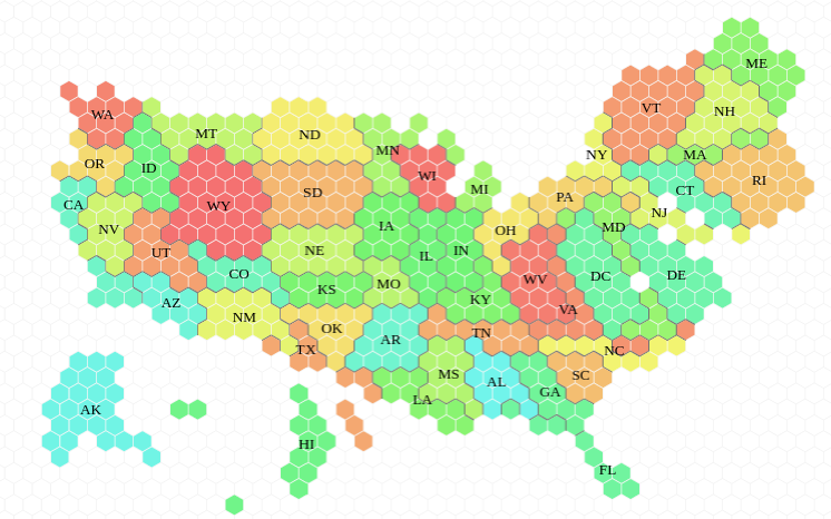
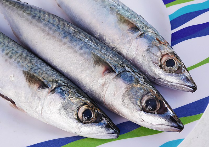
Cette semaine, l’énigme “classique” de FiveThirtyEight (qu’on peut retrouver ici) demande de trouver des mots n’ayant aucune lettre en commun avec un et seul état américain. Par exemple, “mackerel” (le maquereau) a des lettres en commun avec tous les états sauf l’Ohio.

Ce problème peut s’adapter au cas français : quels sont les mots n’ayant aucune lettre en commun avec un et un seul département français ?

En reprenant la liste de mots utilisés pour notre article sur Motus et sur “Des Chiffres et des Lettres”, qui sont de 10 lettres au maximum (selon les règles des jeux), on trouve plus de 15 000 mots qui répondent à notre définition ! L’un d’entre eux est d’ailleurs “MAQUEREAUX”, qui partage (au moins) une lettre en commun avec tous les départements, sauf le Lot.

C’est d’ailleurs ce département qui est le plus souvent à l’origine de la présence des mots dans la liste ; c’est assez logique, car il ne contient ni A, ni E, ni I (lettres qui sont très présentes dans les autres départements), et ne contient que trois lettres.

En utilisant le dictionnaire Lexique, on peut chercher parmi des mots de plus de 10 lettres ceux qui répondent à notre définition. Le mot le plus long répondant à la définition est alors MULTIDIMENSIONNELLE, avec 19 lettres, grâce au département du Var.

Il est possible d’aller plus loin, si l’on accepte de compter tous les caractères des mots et non uniquement les lettres. Dans ce cas, avec 22 signes, le mot répondant à la définition est SUIVEZ-MOI-JEUNE-HOMME (oui, ce mot existe ; non, aucun lien avec les autres maquereaux) car il n’a aucune lettre en commun avec le Gard.

Comment trouver ces mots : description de l’algorithme

Le programme permettant de trouver les mots satisfaisant à la condition demandée (aucune lettre en commun avec un et un seul département) se décompose en plusieurs étapes.

Tout d’abord, on construit des matrices (des tableaux) dont chaque colonne est une lettre de l’alphabet et chaque ligne correspond à, soit un mot du dictionnaire, soit un département. Au croisement d’une ligne et d’une colonne se trouve une indicatrice TRUE/FALSE (qu’on recodera 1/0 après) indiquant si oui ou non la lettre se trouve dans le mot concerné. Pour cela, on utilise la fonction str_detect du package stringR.

sapply(LETTERS,FUN=str_detect,string="AIN")
A     B     C     D     E     F     G     H     I     J     K     L     M     N     O     P 
TRUE FALSE FALSE FALSE FALSE FALSE FALSE FALSE TRUE FALSE FALSE FALSE FALSE TRUE FALSE FALSE 
Q     R     S     T     U     V     W     X     Y     Z 
FALSE FALSE FALSE FALSE FALSE FALSE FALSE FALSE FALSE FALSE 

On a ainsi construit un tableau pour le dictionnaire tableau_dico et un tableau pour les départements tableau_dep. La commande suivante va calculer pour chaque mot du dictionnaire le nombre de département ne partageant aucune lettre en commun.

f <- function(x,ajout) {
  return(max(x + ajout))
}

sum(apply(tableau_dep,MARGIN = 1,f,ajout=tableau_dico[mot,]) == 1))

En décomposant un peu le code :

  • la fonction f construite ici prend deux vecteurs x et ajout et calcule le maximum de la somme des deux vecteurs ;
  • ici, ces deux vecteurs sont la ligne de tableau_dico associée au mot choisi et une ligne de tableau_dep, soit des vecteurs de 0 et 1 suivant si les lettres appartiennent aux mots considérés ;
  • f peut ici renvoyer 1 ou 2 : s’il renvoie 1, cela veut dire qu’il n’y a aucune lettre en commun, sinon, la valeur associée à cette lettre serait de 2, car somme de 1 et 1 dans chacun de deux vecteurs, et donc f calculerait un maximum de 2 ;
  • on applique cette fonction à l’ensemble des départements dans tableau_dep (apply avec le choix de margin=1 pour indiquer que l’on travaille sur les lignes) ;
  • on compte alors le nombre de départements pour lesquels cette sortie est 1.

Une fois qu’on a appliqué cette commande à l’ensemble des mots du dictionnaire, on peut enfin isoler les “maquereaux” en filtrant sur ceux pour lesquels le nombre de départements n’ayant aucune lettre en commun est exactement de 1.

Image : Atlantic mackerels (Petar Milošević)

Rolling some dices

Today, a quick post trying to provide an answer to this week Riddle Classic on FiveThirtyEight :

The fifth edition of Dungeons & Dragons introduced a system of “advantage and disadvantage.” When you roll a die “with advantage,” you roll the die twice and keep the higher result. Rolling “with disadvantage” is similar, except you keep the lower result instead. The rules further specify that when a player rolls with both advantage and disadvantage, they cancel out, and the player rolls a single die. Yawn!

There are two other, more mathematically interesting ways that advantage and disadvantage could be combined. First, you could have “advantage of disadvantage,” meaning you roll twice with disadvantage and then keep the higher result. Or, you could have “disadvantage of advantage,” meaning you roll twice with advantage and then keep the lower result. With a fair 20-sided die, which situation produces the highest expected roll: advantage of disadvantage, disadvantage of advantage or rolling a single die?

Extra Credit: Instead of maximizing your expected roll, suppose you need to roll N or better with your 20-sided die. For each value of N, is it better to use advantage of disadvantage, disadvantage of advantage or rolling a single die?

This problem is quite similar to some issues we’ve already tackled on this website, such as Tennis vs Badminton, or archery points (FR), or even how Eurovision rules impacts french rankings (FR). In order to answer we’re going to use simulations with R. The main set of functions needed is described here:

dice <- function() {return(sample(1:20,1))}

advantage <- function() {
  a <- dice()
  b <- dice()
  return(max(a,b))
} 

disadvantage <- function() {
  a <- dice()
  b <- dice()
  return(min(a,b))
} 

disadvantage_of_advantage <- function() {
   a <- advantage()
   b <- advantage()
   return(min(a,b))
 }

advantage_of_disadvantage <- function() {
   a <- disadvantage()
   b <- disadvantage()
   return(max(a,b))
 } 

Then, we just need to simulate a fair amount (say, n = 10 000 or 100 000) of every dice rolling method. The first question to answer is: how to get the best rolls on average? The following graph answers it nicely, showing that the “disadvantage of advantage” method leads to better results than just rolling a dice, and even better ones than “advantage of disadvantage”.

Will this method be efficient for the other problem, which is maximising our chances to roll a value higher than a set threshold (resulting in harming the dragon, for instance, instead of failing miserably in our attempt)? The answer is yes… but only for lower values of the threshold!

As shown by the graph, as long as the threshold is 14 or higher (and killing a dragon might be that hard!), it’s better to just roll a dice. Why? That’s because our advantage and disadvantage modifiers tend to concentrate the distributions of values obtained: getting a 20 on “disadvantage of advantage” means that you need to get a 20 on both previous rollings with advantage, meaning that you need at least one 20 during each one ; this is extremly unlikely!

Riddler and Voter Power Index

Oliver Roeder has a nice puzzle: the riddler. Just like last week, this week’s puzzle has an interesting application to the US Election and I enjoyed it really much, so I figured I might just write a blog post 🙂 In this article, we’ll solve this week’s riddler two different ways (just because :p) and discuss an indicator used on FiveThirtyEight’s prediction model for the election: the Voter Power Index.

Exact solution and Stirling approximation

I won’t write again the problem and notations, but you can find them here. We’ll also assume N is odd (as precised later by Ollie on Twitter). This assumption won’t matter much because we’ll only look at applications for large values of N. Let’s write:

\(\mathbb{P} = \Pr(you~decide~the~election)\)


Your vote is obviously going to be decisive if there is a tie between the N-1 other votes (convienently, N-1 is even). The votes are all independant with same probability p=1/2, so they are Bernoulli trials. Consequently, the probability we’re looking for is the probability that exactly half of these Bernoulli trial succeed, which is by definition the binomial distribution. Thus:

\(\mathbb{P} = {{N-1}\choose{\frac{N-1}{2}}} p^{\frac{N-1}{2}} {(1-p)}^{\frac{N-1}{2}} \)


As p=0.5, the exact value for the probability of your vote being decisive is thus:

\(\fbox{$\mathbb{P} = \frac{{{N-1}\choose{\frac{N-1}{2}}}}{{2}^{N-1}}$}\)


So, here is the exact solution, but it’s not super useful as is. Much more interesting is how this varies with N (with N sufficiently large). We can use Stirling’s approximation:

\(\log \mathbb{P} = \log {{N-1}\choose{\frac{N-1}{2}}} – (N-1) \log 2 \\
~~~~\sim N \log N – \frac{N}{2} \log \frac{N}{2} – \frac{N}{2} \log \frac{N}{2} + \frac{1}{2} \left( \log N – \log \frac{N}{2} \\~~~~~~~- \log \frac{N}{2} – \log 2\pi \right) – N \log 2 \\~~~~\sim – \frac{1}{2} \log N + \log 2 – \frac{1}{2} \log 2\pi \)

Thus for sufficiently large N, the probability your vote is the decisive vote varies like the inverse of the square root of N:

\(\fbox{$\mathbb{P}\sim \sqrt{\frac{2}{N\pi}} \approx \frac{0.8}{\sqrt{N}}$}\)

A very simple solution for large N

Actually, we could have obtained this result for large N much more simply. We know that asymptotically the binomial distribution is gonna converge to a normal distribution. The event that your vote is the decisive one is actually the most probable event, as probabilities that the other people vote for either candidates are equal to 1/2. So the solution to the riddler can be easily computed using the density of the normal distribution:

\(\mathbb{P} = \phi(0) = \frac{1}{\sqrt{2\pi \sigma^2}}\)

with:

\(\sigma^2 = Np(1-p) = \frac{N}{4}\)

(the variance of the binomial distribution), we get the same result as in the first paragraph:

\(\fbox{$\mathbb{P}\sim \sqrt{\frac{2}{N\pi}} \approx \frac{0.8}{\sqrt{N}}$}\)

Mode of normal distribution for various standard deviations. © W. R. Leo

Voter Power Index

Caption from FiveThirtyEight's model
Caption from FiveThirtyEight’s model

In the US Presidential election, voters don’t elect directly their preferred candidates, but “electors” who will eventually get to vote for the president. For example, California get 55 electors while Wyoming only get 3. But divided by the number of voters in each of these states, it appears that there are approximately 510 000 voters for each elector in California while only 150 000 voters get to decide an electoral vote in Wyoming. If we assumed that probabilities of voting for each candidate was equal in these states, we can use our formula to get the relative likelihood that one vote is going to change the outcome in the election in these two states:

\(\sqrt{\frac{510000}{150000}} \approx 1.8\)

So in a way, a vote by a Californian is nearly 2 times less important than a vote cast in Wyoming!

Of course, probabilities are far from being equal for this year’s 2 candidates in California and Wyoming. And as Michael Vartan noted, the value of this probability matters very much!

All parameters taken into account (also including the different configurations of the electoral college in other states), this is what Nate Silver call the Voter Power Index. For this year, the probabilities that one vote will change the outcome of the whole election is highest in New Hampshire and lowest in DC.

Featured image: Number of electoral votes per voter for each state. Made using the awesome tilegram app