Being able to make causal claims is a key business value for any data science team, no matter their size.
Quick analytics (in other words, descriptive statistics) are the bread and butter of any good data analyst working on quick cycles with their product team to understand their users. But sometimes some important questions arise that need more precise answers. Business value sometimes means distinguishing what is true insights from what is incidental noise. Insights that will hold up versus temporary marketing material. In other terms causation.
When answering these questions, absolute rigour is required. Failing to understand key mechanisms could mean missing out on important findings, rolling out the wrong version of a product, and eventually costing your business millions of dollars, or crucial opportunities.
Ron Kohavi, former director of the experimentation team at Microsoft, has a famous example: changing the place where credit card offers were displayed on amazon.com generated millions in revenue for the company.
The tech industry has picked up on this trend in the last 6 years, making Causal Inference a hot topic in data science. Netflix, Microsoft and Google all have entire teams built around some variations of causal methods. Causal analysis is also (finally!) gaining a lot of traction in pure AI fields. Having an idea of what causal inference methods can do for you and for your business is thus becoming more and more important.
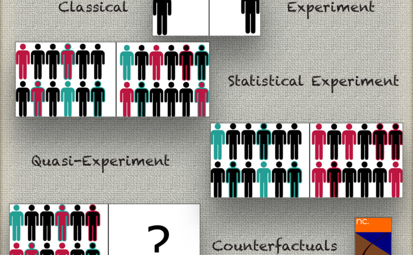
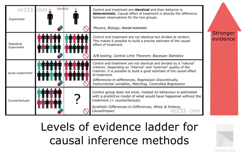
The causal inference levels of evidence ladder
Hence the causal inference ladder cheat sheet! Beyond the value for data scientists themselves, I’ve also had success in the past showing this slide to internal clients to explain how we were processing the data and making conclusions.
The “ladder” classification explains the level of proof each method will give you. The higher, the easier it will be to make sure the results from your methods are true results and reproducible – the downside is that the set-up for the experiment will be more complex. For example, setting up an A/B test typically requires a dedicated framework and engineering resources.
Methods further down the ladder will require less effort on the set-up (think: observational data), but more effort on the rigour of the analysis. Making sure your analysis has true findings and is not just commenting some noise (or worse, is plain wrong) is a process called robustness checks. It’s arguably the most important part of any causal analysis method. The further down on the ladder your method is, the more robustness checks I’ll require if I’m your reviewer 🙂
I also want to stress that methods on lower rungs are not less valuable – it’s almost the contrary! They are brilliant methods that allow use of observational data to make conclusions, and I would not be surprised if people like Susan Athey and Guido Imbens, who have made significant contributions to these methods in the last 10 years, were awarded the Nobel prize one of these days!
Rung 1 – Scientific experiments
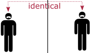
On the first rung of the ladder sit typical scientific experiments. The kind you were probably taught in middle or even elementary school. To explain how a scientific experiment should be conducted, my biology teacher had us take seeds from a box, divide them into two groups and plant them in two jars. The teacher insisted that we made the conditions in the two jars completely identical: same number of seeds, same moistening of the ground, etc.
The goal was to measure the effect of light on plant growth, so we put one of our jars near a window and locked the other one in a closet. Two weeks later, all our jars close to the window had nice little buds, while the ones we left in the closet barely had grown at all.
The exposure to light being the only difference between the two jars, the teacher explained, we were allowed to conclude that light deprivation caused plants to not grow.
Sounds simple enough? Well, this is basically the most rigorous you can be when you want to attribute cause. The bad news is that this methodology only applies when you have a certain level of control on both your treatment group (the one who receives light) and your control group (the one in the cupboard). Enough control at least that all conditions are strictly identical but the one parameter you’re experimenting with (light in this case). Obviously, this doesn’t apply in social sciences nor in data science.
Then why do I include it in this article you might ask? Well, basically because this is the reference method. All causal inference methods are in a way hacks designed to reproduce this simple methodology in conditions where you shouldn’t be able to make conclusions if you followed strictly the rules explained by your middle school teacher.
Rung 2 – Statistical Experiments (aka A/B tests)

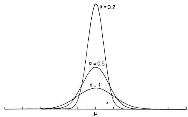
Probably the most well-known causal inference method in tech: A/B tests, a.k.a Randomized Controlled Trials for our Biostatistics friends. The idea behind statistical experiments is to rely on randomness and sample size to mitigate the inability to put your treatment and control groups in the exact same conditions. Fundamental statistical theorems like the law of large numbers, the Central Limit theorem or Bayesian inference gives guarantees that this will work and a way to deduce estimates and their precision from the data you collect.
Arguably, an Experiments platform should be one of the first projects any Data Science team should invest in (once all the foundational levels are in place, of course). The impact of setting up an experiments culture in tech companies has been very well documented and has earned companies like Google, Amazon, Microsoft, etc. billions of dollars.
Of course, despite being pretty reliable on paper, A/B tests come with their own sets of caveats. This white paper by Ron Kohavi and other founding members of the Experiments Platform at Microsoft is very useful.
Rung 3 – Quasi-Experiments

As awesome as A/B tests (or RCTs) can be, in some situations they just can’t be performed. This might happen because of lack of tooling (a common case in tech is when a specific framework lacks the proper tools to set up an experiment super quickly and the test becomes counter-productive), ethical concerns, or just simply because you want to study some data ex-post. Fortunately for you if you’re in one of those situations, some methods exist to still be able to get causal estimates of a factor. In rung 3 we talk about the fascinating world of quasi-experiments (also called natural experiments).
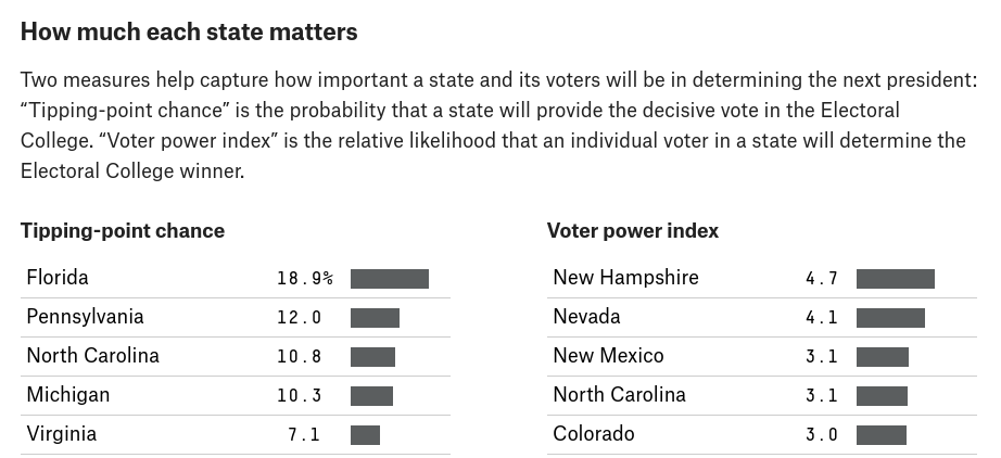
A quasi-experiment is the situation when your treatment and control group are divided by a natural process that is not truly random but can be considered close enough to compute estimates. In practice, this means that you will have different methods that will correspond to different assumptions about how “close” you are to the A/B test situation. Among famous examples of natural experiments: using the Vietnam war draft lottery to estimate the impact of being a veteran on your earnings, or the border between New Jersey and Pennsylvania to study the effect of minimum wages on the economy.
Now let me give you a fair warning: when you start looking for quasi-experiments, you can quickly become obsessed by it and start thinking about clever data collection in improbable places… Now you can’t say you haven’t been warned 😜 I have more than a few friends who were lured into attracted by a career in econometrics for the sheer love of natural experiments.
Most popular methods in the world of quasi-experiments are: differences-in-differences (the most common one, according to Scott Cunnigham, author of the Causal Inference Mixtape), Regression Discontinuity Design, Matching, or Instrumental variables (which is an absolutely brilliant construct, but rarely useful in practice). If you’re able to observe (i.e. gather data) on all factors that explain how treatment and control are separated, then a simple linear regression including all factors will give good results.
Rung 4 – The world of counterfactuals

Finally, you will sometimes want to try to detect causal factors from data that is purely observational. A classic example in tech is estimating the effect of a new feature when no A/B test was done and you don’t have any kind of group that isn’t receiving the feature that you could use as a control:
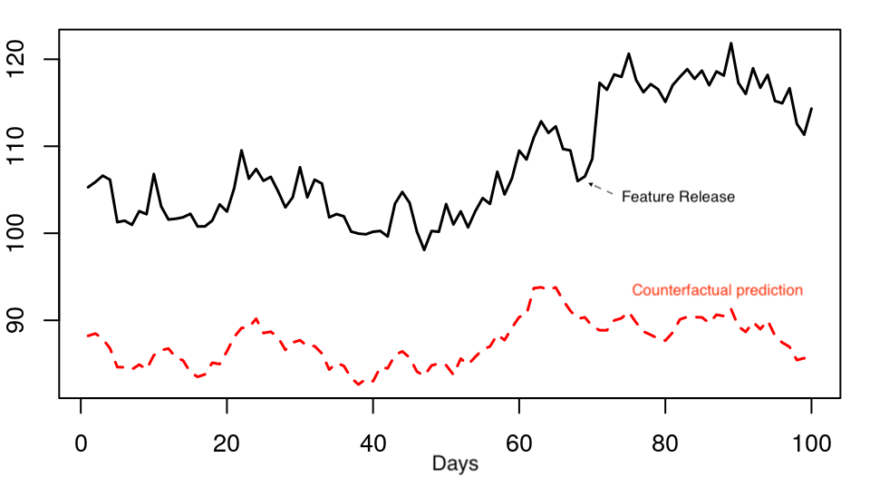
Maybe right new you’re thinking: wait… are you saying we can simply look at the data before and after and be allowed to make conclusions? Well, the trick is that often it isn’t that simple to make a rigorous analysis or even compute an estimate. The idea here is to create a model that will allow to compute a counterfactual control group. Counterfactual means “what would have happened hadn’t this feature existed”. If you have a model of your number of users that you have enough confidence in to make some robust predictions, then you basically have everything
There is a catch though. When using counterfactual methods, the quality of your prediction is key. Without getting too much into the technical details, this means that your model not only has to be accurate enough, but also needs to “understand” what underlying factors are driving what you currently observe. If a confounding factor that is independent from your newest rollout varies (economic climate for example), you do not want to attribute this change to your feature. Your model needs to understand this as well if you want to be able to make causal claims.
This is why robustness checks are so important when using counterfactuals. Some cool Causal Inference libraries like Microsoft’s doWhy do these checks automagically for you 😲 Sensitivity methods like the one implemented in the R package tipr can be also very useful to check some assumptions. Finally, how could I write a full article on causal inference without mentioning DAGs? They are a widely used tool to state your assumptions, especially in the case of rung 4 methods.
(Quick side note: right now with the unprecedented Covid-19 crisis, it’s likely that most prediction models used in various applications are way off. Obviously, those cannot be used for counterfactual causal analysis)
Technically speaking, rung 4 methods look really much like methods from rung 3, with some small tweaks. For example, synthetic diff-in-diff is a combination of diff-in-diff and matching. For time series data, CausalImpact is a very cool and well-known R package. causalTree is another interesting approach worth looking at. More generally, models carefully crafted with domain expertise and rigorously tested are the best tools to do Causal Inference with only counterfactual control groups.
Hope this cheat sheet will help you find the right method for your causal analyses and be impactful for your business! Let us know about your best #causalwins on our Twitter, or in the comments!


![[Sampling] Talk at INSPS – Avignon](https://nc233.com/wp-content/uploads/2016/06/Palais_des_Papes_à_Avignon_-825x510.jpg)